본문으로 건너뛰기

데이터 가치평가 및 데이터 자산화 (Data Valuation & Assetization)

· 약 3분

데이터 가치평가 및 데이터 자산화의 개요

데이터 가치평가 및 데이터 자산화의 개념

  • 데이터 가치평가: 데이터산업법에 의거, 대상 데이터의 활용을 통해 창출할 수 있는 경제적 가치를 가치평가 방법론을 적용하여 정량적 화폐가치로 산정하는 체계.
  • 데이터 자산화: 기업 내 고립된 데이터를 단순 정보(Information) 수준을 넘어 비즈니스 가치를 반복 창출할 수 있는 경영 전략 자산(Asset)으로 정의, 관리, 운용하는 일련의 과정.

데이터의 자산적 가치 창출 배경 (필요성)

  • 자금 조달 다변화: 디지털 자산화 도래에 따라 데이터를 담보로 한 금융 보증, 대출 및 투자 유치 활성화.
  • 데이터 비즈니스 모델 구축: 데이터 거래소 활성화에 따른 라이선싱 가격 산정 표준 기준 요구.

데이터 가치평가의 개념과 가치평가 방법론

데이터 경제적 가치평가 체계도

데이터 가치평가의 3대 방법론 비교

구분수익접근법 (Income Approach)원가 및 시장접근법 (Cost/Market)
개념데이터 활용으로 인한 미래 기대 수익을 현재 가치로 할인생성에 소요된 비용 또는 시장 거래 사례 기반 산정
평가 대상사업적 완성도가 높고 현금 흐름 예측이 가능한 데이터거래 사례가 존재하거나 대체 구축 비용 산정이 용이한 데이터
핵심 원리DCF법 및 데이터 기여율(DRDR) 반영:
V=t=1nCFt×DRt(1+r)tV = \sum_{t=1}^{n} \frac{CF_t \times DR_t}{(1 + r)^t}
- 대체원가 계산 (역사적 원가 적용)
- 유사 거래 사례 비교 (배수법 적용)
주요 한계미래 현금 흐름 및 데이터 기여율의 임의 추정 위험성데이터 독창성으로 인한 거래 사례 부재, 미래 가치 미반영

데이터 자산화의 개념과 핵심요소 및 라이프사이클

데이터 자산화의 개념 및 거버넌스 체계

  • 데이터를 자산화하기 위해서는 데이터의 품질, 표준, 메타데이터를 통합 관리하는 데이터 거버넌스(원칙, 조직, 프로세스) 체계가 전제되어야 함.

데이터 자산화의 핵심 구성요소 및 라이프사이클

구분핵심요소 및 라이프사이클세부 설명 및 산출물
가치 식별데이터 가치평가 체계비즈니스 관련성 분석을 통해 자산화 대상 코어 데이터 선별
구조화데이터 제품화 (Data Product)실무자가 즉시 활용 가능하도록 API, 대시보드 형태로 패키징
관리 통제데이터 카탈로그 및 계보메타데이터 기반 리니지(Lineage) 관리로 투명성과 품질 보장
주기 관리데이터 라이프사이클생성 ➡️ 저장 ➡️ 분석 ➡️ 활용 ➡️ 아카이빙/폐기의 단계별 통제

데이터 가치평가 및 데이터 자산화의 활용사례 및 고려사항

데이터 가치평가 및 자산화의 실무적 활용사례

구분내용 (활용 분야)비고 (실제 사례)
금융 및 보증데이터 담보 보증서 발급 및 보증 대출신용보증기금, 기술보증기금 주도의 가치평가 연계 금융 지원
자산 및 매각기업 M&A 및 투자 유치 시 자산 가치 평가기업 보유 독점 데이터의 가치를 기업가치(Valuation)에 합산
거래 및 중개데이터 거래소 기반 데이터 판매 및 라이선싱금융·교통·통신 분야 이종 데이터 결합 및 API 판매 거래

성공적인 데이터 자산화를 위한 고려사항

  • 컴플라이언스 준수: 개인정보보호법에 의거, 가명 정보 처리 및 개인 식별 방지 필터링을 통해 법적 안정성을 확보해야 함.
  • 데이터 리터러시 내재화: 조직 전반이 데이터를 이해하고 분석·활용할 수 있는 CDO 중심의 역량 내재화 프로세스가 결합되어야 실현

CNN 012

· 약 6분
  • Three main layers of a CNN
    • CONV: Convolution Layer
    • POOL: Pooling Layer
    • FC: Fully Connected Layer
    • CONV extracts features, POOL downsamples feature maps, and FC makes the final prediction.
  • Why CNNs use over ANNs for image processing
    • Computationally efficient
    • Using Filters to capture spatial features
    • Sharing weights across the image
  • Overfitting
    • The model essentially memorizes the training data, leading to poor performance on unseen data
    • To prevent overfitting, we can use techniques like:
      • Dropout: Randomly dropping out neurons during training to prevent co-adaptation
      • Batch Normalization: Normalizing the inputs of each layer to stabilize learning
      • L1/L2 Regularization: Adding a penalty to the loss function to discourage large weights
        • L1 regularization adds a penalty based on the absolute value of the weights (can be zero, can make model sparse and useful for feature selection.)
        • L2 regularization adds a penalty based on the squared value of the weights (not can be zero, reduce model complexity and overfitting.)
      • Data Augmentation: Creating new training samples by applying transformations to existing data
  • ReLU
    • If the input is below zero, ReLU does output 0.
    • If the input is above zero, it outputs the input value itself.
    • max(0, x)
    • ReLU can output any number from 0 to infinity, which allows it to capture a wide range of features in the data.
    • It fixes gradient vanishing problem by allowing gradients to flow through the network without being squashed to zero, which can happen with activation functions like sigmoid or tanh.
  • Sigmoid: Binary Classification
  • Softmax: Multi-class Classification
  • Backpropagation: sends the error backward through the network and calculates gradients, so the model knows how to update its weights and biases.
  • Gradient Descent
    • It uses Backpropagation to calculate the exact slope (the gradient) of the error (loss).
    • Then it takes a step in the opposite direction of the gradient to minimize the error.
    • It repeats this interative process until it reaches a local minimum.
  • Vanishing Gradient Problem
    • The gradient becomes too small, so earlier layers learn very slowly or almost stop learning.
    • ReLU helps mitigate this problem by allowing gradients to flow through the network without being squashed to zero.
  • Learning Rate α\alpha
    • It's a hyperparameter that controls how big of a step the model takes down the slope.
    • If α\alpha is too small, the model will take tiny steps and may take a long time to converge.
    • If α\alpha is too large, the model may overshoot the minimum and diverge.
  • Precision: TPTP+FP\frac{TP}{TP + FP}
    • Of all the patients the model predicted as having the disease, how many actually have the disease?
  • Recall: TPTP+FN\frac{TP}{TP + FN}
    • Of all the patients who actually have the disease, how many did the model successfully catch?
    • Recall is more important in medical diagnosis because we want to minimize false negatives (missing a disease).
  • Sliding Window
    • Computationally expensive because it requires multiple passes over the image with different window sizes and strides.
    • Multiple scales are needed to detect objects of varying sizes, which further increases the computational cost.
  • Stride: controls the step size of the sliding filter. Larger stride means smaller output.
  • Edge
    • The points or pixels in an image where brightness or intensities change sharply.
    • Sobel filter
    • Prewitt filter
    • Canny edge detector
  • Padding: adds zeros around the image so the CONV does not shrink the feature map too much.
  • Keep the output dimension the same as the input dimension, we can use padding.
    • P=F12P = \frac{F - 1}{2}
  • Image Classification: Assigning a label to an entire image (e.g., cat, dog, car).
  • Object Detection: Identifying and localizing multiple objects within an image (e.g., bounding boxes)
  • Instance Segmentation: Identifying and segmenting each object instance in an image (e.g., pixel-level masks)
  • Momentum: uses an exponentially weighted average of past gradients to smooth updates and accelerate convergence.
  • RMSProp: uses an exponentially weighted average of squared gradients to adapt the learning rate for each parameter.
  • Adam: combines Momentum and RMSProp by using both the first moment, average gradient, and the second moment, average squared gradient.
  • Hyperparameters: learning rate, batch size, number of epochs, optimizer type, dropout rate, etc.
  • Supervised Learning: The model learns from labeled data, classification, regression.
  • Unsupervised Learning: The model learns from unlabeled data, clustering.
  • Loss/Cost function: an estimate of how far the model's predictions are from the actual target/answer.
  • AI is a broad concept of machines performing human-like tasks.
  • ML is a subset of AI that learns from data
  • DL is a subset of ML that uses deep neural networks with many layers.
  • ML's major problem
    • insufficient data
    • non-representative training data
    • poor-quality data
    • irrelevant features
    • overfitting
    • underfitting
  • When we use ML?
    • a large amount of data for finding patterns and making predictions
    • too many rules or too much complexity for humans to handle
  • Faster R-CNN: Propose regions first, then classify them
    • RPN: Region Proposal Network, which generates candidate object proposals
  • YOLO: Predict boxes and class probabilities directly from the image in one pass
    • Anchor boxes: predefined bounding boxes of different sizes and aspect ratios used to predict the location of objects in YOLO.
  • NMS: Non-Maximum Suppression, selects the best bounding box among overlapping boxes based on confidence scores.
  • 1×1 convolution mixes channel information and can reduce the number of channels, so later convolutions become cheaper.
  • Inception module: learns small, medium, and large visual features at the same time.
  • Transfer Learning Strategies:
    • First, if the new dataset is small and similar to the original dataset, we can use the pre-trained model directly.
    • Second, if the dataset is similar but has different classes, we freeze the convolutional layers and train only the fully connected classification layer.
    • Third, if the dataset is small but not very similar, we freeze the early convolutional layers and fine-tune the later convolutional layers plus the FC layer.
    • Finally, if the dataset is large and different, we can fine-tune the whole network.
  • IoU: Intersection over Union, a metric used to evaluate the accuracy of object detection models by comparing the predicted bounding box with the ground truth bounding box.

CNN 011

· 약 4분

Sequence

  • has a lot of context to predict the next behavior

Sequence modelling types

  • One to One Binary classification
    • X -> Y'
    • Will it rain today? Yes/No
  • Many to One Sentiment Analysis
    • X1, X2, X3, ... -> Y'
    • Is this review positive or negative?
  • One to Many Image Captioning
    • X -> Y1, Y2, Y3, ...
    • Image: A Women is throwing a frisbee in the park
  • Many to Many Q&A with LLMs, Language translations
    • X1, X2, X3, ... -> Y1, Y2, Y3, ...
    • Q: Hey, Siri How's the weather today? A: It's sunny and warm outside.

RNN

Recurrent Neural Network

  • yt=f(xt,ht1)y'-t = f(x_t, h_{t-1})
    • yty'-t: output at time t
    • xtx_t: input at time t
    • ht1h_{t-1}: Past momery

Sequence Modelling

  • Support for Variable-Length input
  • Has Temploral Dependency (Long, Short-term)
  • Preserve the information order
  • Share parameters across sequence

Attention

  • Why
    • RNNs process sequences one step at a time
    • Long sentences lead to Long-term memory loss
    • Important words can be hidden in long dependencies
  • Attention helps to focus on relevant parts of the input
  • For each output word, atention decides which input word is most important
  • Computes a weighted sum of all input vectors
  • Higher weights words are more important

Transformer

  • Self-Attention is the foundation for Transformers architecture
  • Entire sequence is processed in parallel
  • Has Encoder and Decoder block
  • Stack of Layers with Self Attention and Feed Forward Neural Network

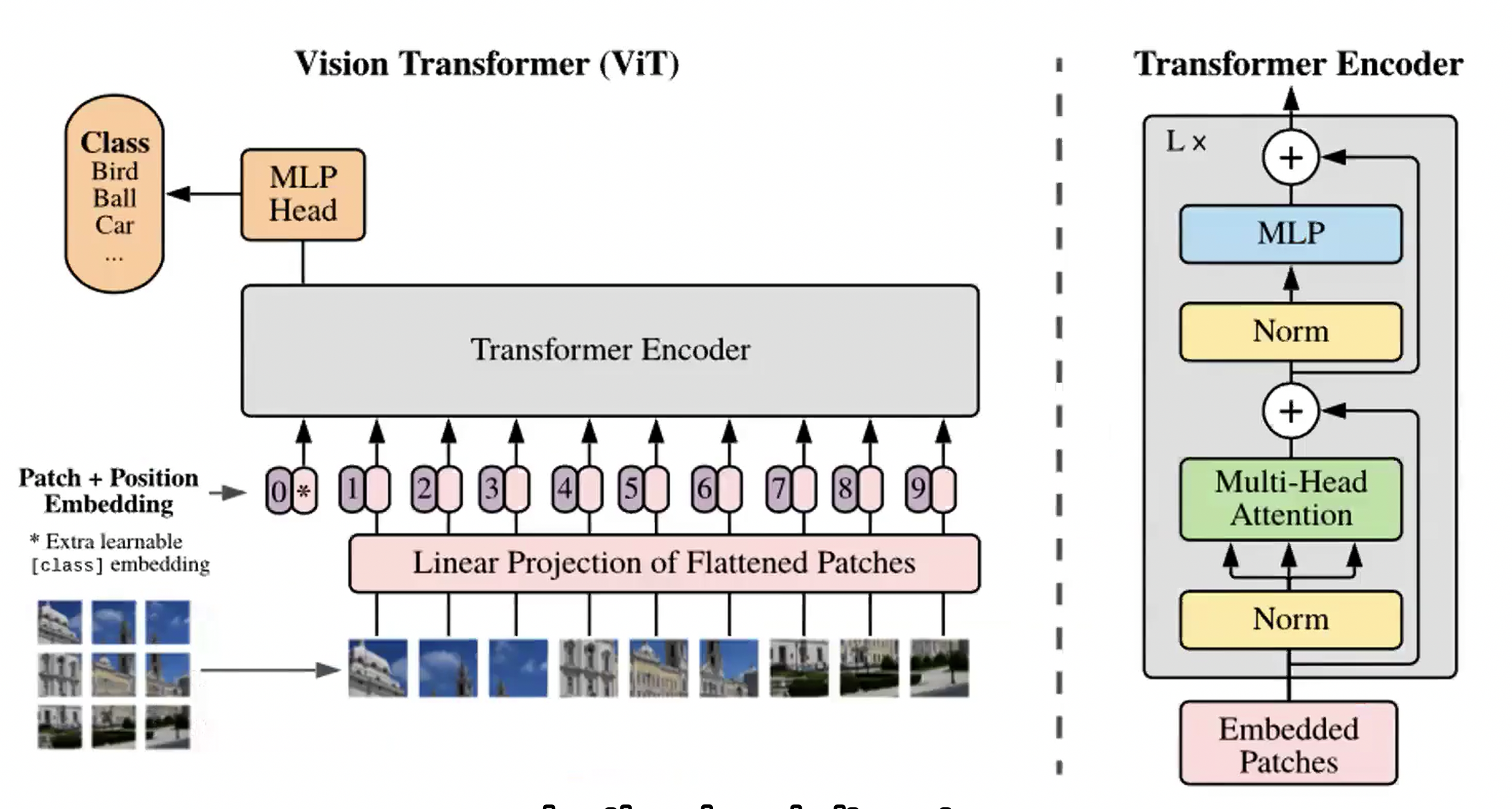
Vision Image Transformer (ViT)

  • Vision transformer have extensive application in all computer vision tasks
  • ViT looks at images, like how lanauge model looks at words
  • Image are represented as sequence of patches

Steps to use ViT

  1. Split an image into patches
  2. Flatten the patches
  3. Produce lower-dimensional linear embeddings from the flattened patches
  4. Add positional embeddings
  5. Feed the sequence as input to a standard transformer encoder
  6. Pretrain the model with image labels (fully supervised on a huge dataset)
  7. Finetune on the downstream dataset for image classification

ViT

CNNs vs Vision Transformer (ViT)

Key AspectsCNNsViT
Input HandlingProcesses the entire image using filters (kernels)Splits image into fixed-size patches (like tokens)
Local vs. GlobalFocuses on local patterns first (edges, textures)Uses global self-attention to relate all patches
ArchitectureHierarchical (convs -> pools -> deeper features)Flat transformer encoder stack
Training Data NeedWorks well with limited dataNeeds lots of data or pretraining
ComputationEfficient with low-res inputsComputationally heavier, especially on large images
ParallelismLimited; uses sequential feature stackingHigh; patch processing is highly parallelizable

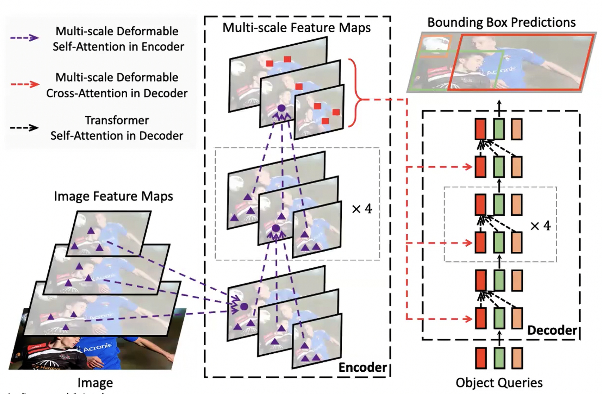
RF-DETR

Roboflow Detection Transformer

  • Object detection techniques using Transformers
  • An improvement over the original DETR (Detection Transformer) model
  • DETR looks at everything globally but miss small things.
  • RF-DETR looks globally and understands the relationships between things.
  • First real-time Transformer-based object detection architecture
  • Outperforms all object detection models, 60+% mAP on COCO dataset

RF-DETR

Diffusion Models

  • Generate new data samples (images, audio, text) that is similar to a training dataset by learning to reverse a gradual noise process
  • Forward Diffusion
    • Add noise gradually to the original image for many steps
    • Iterate until the image becomes pure noise
    • Gaussian noise used (no learning)
  • Reverse Diffusion
    • Denosing, model is trained to predict and reverse this noise
    • Use the prediction to denoise the image
    • Given a noisy image, it predicts a slightly less noisy image version
    • After several steps, it reconstructs a clean and new image from pure noise

Steps to train a diffusion model

  1. Start with real data
  2. Add noise step by step, until the image becomes pure noise
  3. Train a model to reverse this process, denoising to recover the original image
  4. Once trained, the model can start from pure noise and generate new and realistic samples

Applications of Diffusion Models

  • Given a lof of sprite sample images
  • Can generate New sprite images
    • New image generation from image input

CNN 010

· 약 5분

Drawbacks of Anchor-based detectors

It is sensitive to:

  • Size
  • Aspect Ratio
  • Number of Anchor boxes (Fixed)
  • To much variation with shape
  • Small object
  • May not generalize due to pre-defined anchor boxes
  • Computation expensive

Anchor-free detectors

  • Localize objects without using boxes as proposals
  1. Key-point based
  2. Center-based

Key-point based

  • Locates key object parts in an image
  • Detects spatial locations or points unique to an object
  • With human body as an example
  • Key part of face: nose, eyes, eyebrows, mouth ...
  • Key point of human body: joints, elbows, knees ...
  • Object is represented using Key-points

Center-based

  • Finds positives in the center
  • Predicts four distances from the positive to the potential object boundary
    • Top, left, bottom, right
    • {x, y, T, R, B, L}

YOLO

  • Yolo V1: 2015
    • darknet backbone
  • Yolo V2: 2016
    • Anchor boxes
    • Batch normalization
  • Yolo V3: 2018
    • Objectness score
    • improvement for small objects
  • Yolo V4/V5: 2020
    • Solid Baseline Model
    • Lightweight and Fast
    • image classification, object detection, and instance segmentation
    • Multiple input processing (Video, Image, Live stream)
    • Optimize weights
    • Developed by Ultralytics (not original author)
  • Yolo X/R: 2021
    • Decoupled head
    • First version of Anchor free
    • Improvement efficiency in backbone
  • Yolo V6/V7: 2022
    • Faster and more accurate
  • Yolo NAS/V8: 2023
    • Anchor free
    • Architectural improvement
    • Strong baseline for realtime object detection
  • Yolo V9/V10/V11: 2024
    • Oriented bounding box
    • Strong baseline for oriented object detection
  • Yolo V12: 2025
    • Attention mechanism, introduced transformer
    • Little slower
  • Yolo 26: 2026
    • Deployment on a small form factor hardware
    • realtime object detection on edge devices
    • Strongest baseline for edge device deployment (realtime and accuracy)
    • Efficient Loss Function

YoloX X

  • Anchor-free detector in the Yolo Family
  • Decoupled head used
  • Label assignment using SimOTA
  • Use YoloV3 SPP with DarkNet53 backbone
  • Uses advanced augmentation such as Mix-up & Mosaic
  • Backbone: Feature extraction
  • Neck: Aggregation of multi-scale feature
  • Head: Localization and Classification scores

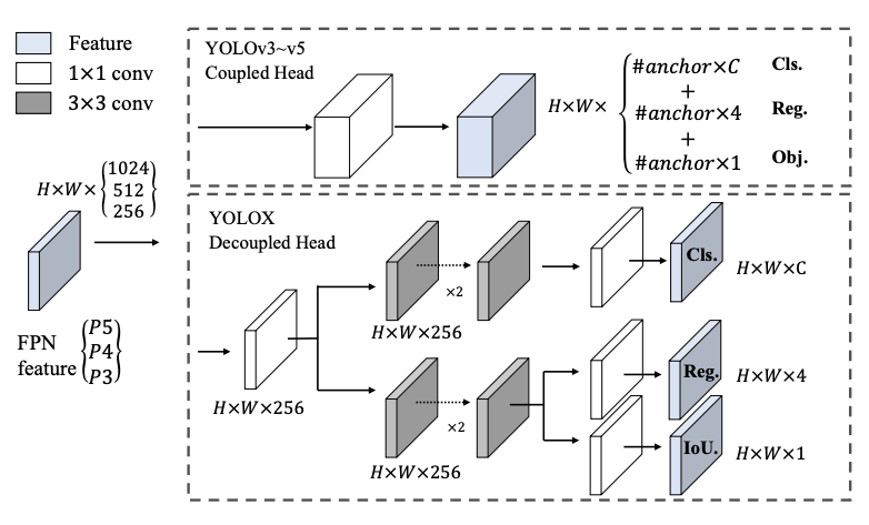
Decoupled head

decoupled head

  • Coupled Head: one head gives regression score and classification score (Dog/Cat + Location, BBox)
  • Decoupled Head:
    • First head gives Classification score (Dog/Cat)
    • Another head gives Regression score (Location, BBox)

Data Augmentation

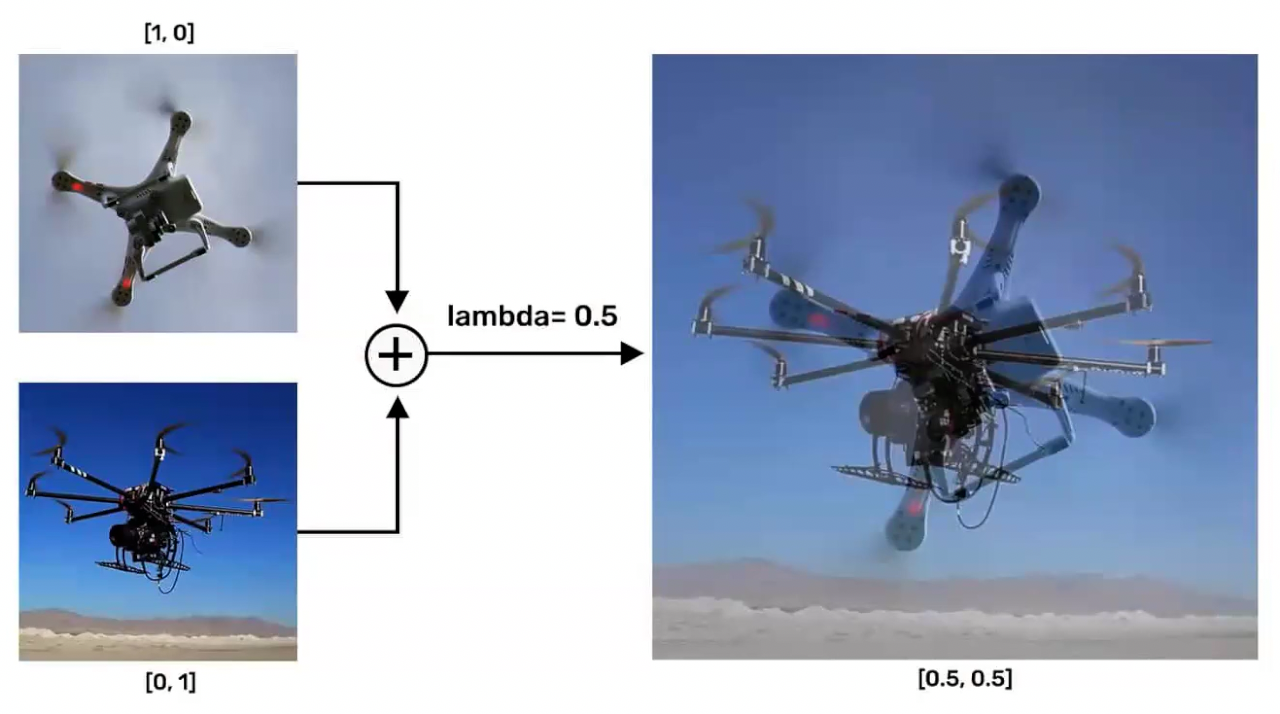
mixup augmentation

  • occluded and overlapped objects
  • improve model robustness

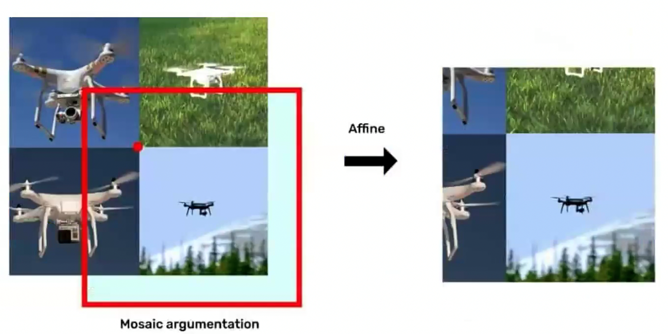
mosaic augmentation

  • four images are combined into one
  • crops and resizes the images to create a new training sample

Yolo 26

  • Realtime computer vision model
  • Detection, Segmentation, Classification, Pose, Tracking, OBB (Oriented Bounding Box)
  • Available in Nano, Small, Medium, Large, XLarge
  • E2E detection pipeline (NMS-free, Non-Maximum Suppression free)
  • Designed for edge AI and fast deployment

Why is it faster

  • NMS-free infrerence removes post-processing overhead
  • Direct bounding box regression (No DFL, Distribution Focal Loss)
  • Lower latency and simpler deploymenet graph
  • CPU-optimized architecture
  • Up to 43% faster on CPUs than V11

Key Changes

  • ProgLoss (Progressive Loss Balancing): improves training stability and convergence
  • STAL (Small-Target-Aware Label Assignment): improves small-object detection
  • MuSGD optimizer improves convergence speed
  • Better speed-accuracy trade-off than many previous YOLO models
  • Ideal for robotics, drones, surveillance, and edge devices

Inference pipeline

  • Backbone: Efficient Hybrid CNN + Attention
  • Neck: PAN-FPN (Multi-scale Feature Fusion)
  • Head (Decoupled & Dual Head)
    • One-to-Many Head: Dense supervision (Traning only, many positives)
    • One-to-One Head: Single best match NMS-free inference (Inference & tranining)

Tranining pipeline

Instance Segmentation

  • Identifies each pixel of an object instance
  • whereas Semantic Segmentation classifies object pixels to specific classes/categories
  • Instance Segmentation
    • SegNet
    • DeepMask
    • SharpMask
    • Mask RCNN
  • Semantic Segmentation
    • Conditional Random Field (CRF)
    • Fully Convolutional Networks (FCN)
    • U-Net
    • Pyramid scene parsing network (PSPNet)

Application of Instance Segmentation

  • Autonomous Driving
  • Scene Understanding
  • Aerial Image Processing

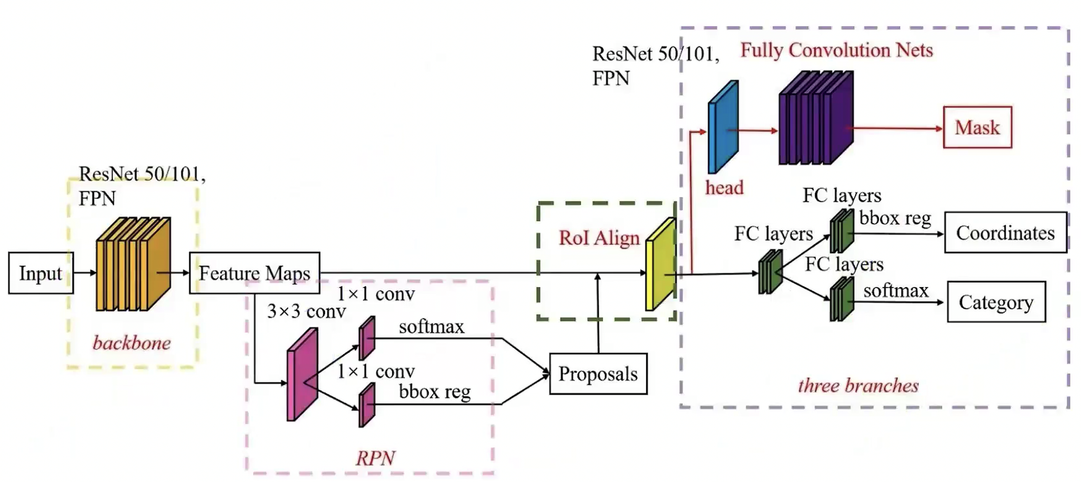
Mask R-CNN

Mask-Region Convolutional Neural Network

  • An addition to the RCNN family, perfoming instance segmentation
  • Improved over Faster RCNN
  • Full Convolutional Network for predicting mask for each class/object.
  • Two stages:
    1. RPN proposes candidiate object bounding boxes
    2. Classify the Candidates, refine bounding boxes, and predict mask.

Mask R-CNN architecture

Limitations of Mask R-CNN

  • Computational Complexity: Traning and inference can be computationally intensive, requiring substantial resources (high resolution images or large datasets).
  • Small-Object Segmentation: may struggle with accurately segment very small objects due to limited pixel information.
  • Data Requirements: Training requires a large amount of annotated data, which can be time-consuming and expensive to acquire.
  • Limited Generalization to Unseen Categories: The model's ability to generalize to unseen object categories is limited.

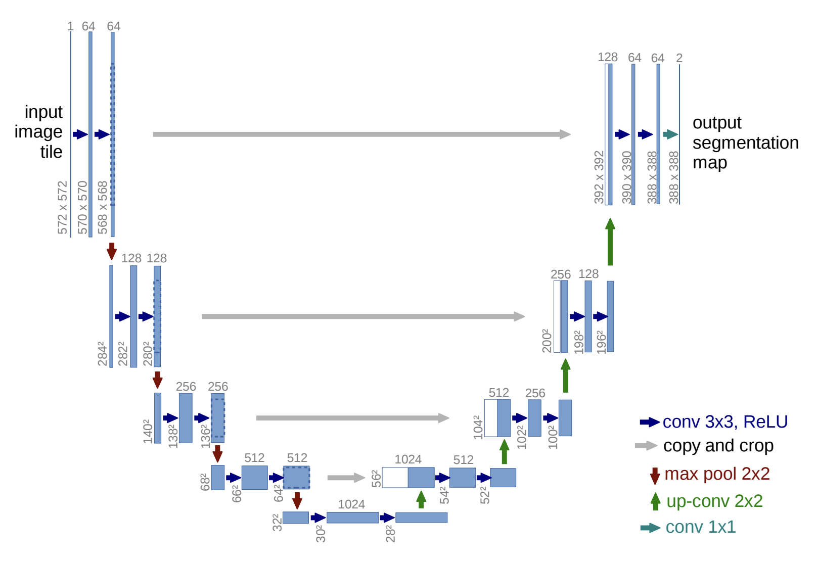
Semantic Segmentation

u-net

  • input image -> u-net -> output segmentation map

References

  • Ge, Z., Liu, S., Wang, F., Li, Z., & Sun, J. (2021). YOLOX: Exceeding YOLO series in 2021. arXiv. https://doi.org/10.48550/arXiv.2107.08430
  • Ronneberger, O., Fischer, P., & Brox, T. (2015). U-Net: Convolutional networks for biomedical image segmentation. In N. Navab, J. Hornegger, W. M. Wells, & A. F. Frangi (Eds.), Medical Image Computing and Computer-Assisted Intervention – MICCAI 2015 (Vol. 9351, pp. 234–241). Springer. https://doi.org/10.1007/978-3-319-24574-4_28

CNN 009

· 약 2분

Prediciting Bounding Boxes

  • Using:
    • Sliding Window (Slow)
    • Selective Search
    • Region Proposals
  • Task:
    • Predict Bouding boxes from CNN

Non Maxima Suppression (NMS)

  1. Check the probabilities of each detection and keep ones with score above a certain threshold (0.7)
  2. For remaining boxes, a. Box with highest score is the detection results. b. Discard any remaining boxes with IoU > 0.5 with final detected box c. i.e. overlap with the box with highest score.

Anchor Boxes

  • Associate each object to:
    • A cell which contains its mid-point and
    • Anchor box for the cell with highest IoU
  • Calculate the IoU of Anchor boxes and prediected Bounding Boxes.
    • IoU(Pbb,Abb)=AreaofOverlapAreaofUnionIoU(P_{bb}, A_{bb}) = \frac{Area of Overlap}{Area of Union}
  • y^={P0,x,y,h,w,C1,C2,P0x,y,h,w,C1,C2}\hat{y} = \{P_0, x, y, h, w, C1, C2, \quad P_0 x, y, h, w, C1, C2\}
    • P0P_0 is objectness score
    • x,yx, y are the coordinates of the center of the bounding box relative to
    • h,wh, w are the height and width of the bounding box
    • C1,C2C1, C2 are the class information for the object in the bounding box

YOLO

  • Real-time performance with 45 FPS, 0.02 sec per image
  • Not suitable for small objects
  • Issues with new or multiple aspect ratios and unable to generalize

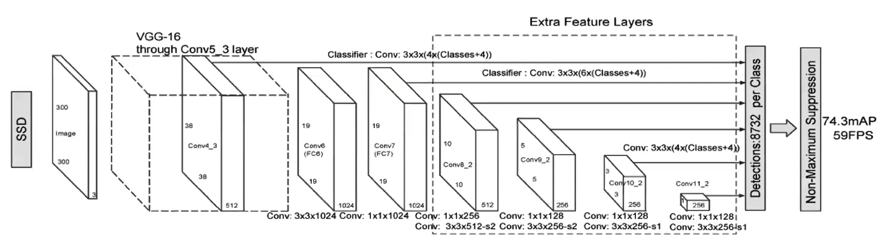
SSD, Single Shot Detector

  • Similar to YOLO, VGG16 base Convolutional Neural Network layers
  • Take advantage of Anchor boxes with different aspect ratios
  • Large number of anchors boxes are chosen
  • Not suitable for small objects
  • 3 times faster than Faster R-CNN
  • with ResNet-101 base SSD may help in detecting small objects with better features from the CONV layers

SSD 300 architecture

Overview of Object Detection

  • Base Networks
    • VGG156
    • ResNet-101
    • Inception-v2, v3
    • ResNet
    • MobileNet
    • Alexnet
    • ZFNet
  • Object Detection Framework
    • R-CNN family
    • YOLO family
    • SSD family
    • F-RCNN family
  • Faster-RCNN is more accurate but slower
  • YOLO/SSD are faster/real-time but may not be very accurate

CNN 008

· 약 4분

Datasets

PASCAL isual Object Classifcation

PASCAL VOC

  • a popular dataset for object detection, classification and segmentation
  • 20 categories

ImageNet

  • a dataset for object detection
  • 500,000 images, 200 categories
  • Not very popular due to large number of classes and size of the dataset

COCO

Microsoft Common Objects in Context dataset

  • a large-scale object detection, segmentation, and captioning dataset.
  • 330,000 images, 80 categories
  • 200,000 labeled images, 1.5 million object instances
  • 91 stuff categories

Intersecxtion over Union (IoU)

IoU=AreaofOverlapAreaofUnionIoU = \frac{Area of Overlap}{Area of Union}

  • a metric used of the evaluation of an object detector
  • how good is the predicted bounding box for an object detected colosely matches

AP

Average Precision

MetricDescription
APAPAP at IoU=.50:0.05:0.95 (primary challenge metric)
APIoU=.50AP^{IoU=.50} AP at IoU=0.50 (PASCAL VOC metric)
APIoU=.75AP^{IoU=.75} AP at IoU=0.75 (strict metric)
APsmallAP^{small}AP for small objects: area<322area < 32^2
APmediumAP^{medium}AP for medium objects: 322<area<96232^2 < area < 96^2
APlargeAP^{large}AP for large objects: area>962area > 96^2
ARmax=1AR^{max=1}AR given 1 detection per image
ARmax=10AR^{max=10}AR given 10 detections per image
ARmax=100AR^{max=100}AR given 100 detections per image
ARsmallAR^{small}AR for small objects: area<322area < 32^2
ARmediumAR^{medium}AR for medium objects: 322<area<96232^2 < area < 96^2
ARlargeAR^{large}AR for large objects: area>962area > 96^2

Taxonomy of Object Detection

History of Object Detection

History of Object Detection

Classification with Localization

  • Classification Task
    • Input: Image
    • Output: Class label
    • Performance Metric: Accuracy
  • Localization Task
    • Input: Image
    • Output: Bounding box coordinates (x,y,Ht,Wd)(x, y, Ht, Wd) or (x,y,x,y)(x, y, x', y')
    • Performance Metric: IoU

Localization Loss

Localization as a regression problem

Detection as a Classification Problem

Region Proposal

  • Find blobs in the image that are most likely to contain objects.
  • Selective Search: ~1000-2000 region proposal using CPU

R-CNN

Region based CNN

  • Convolution Neural Network as feature extractor
  • SVM as classifier
  • Bounding box regression for localization
  • Pass each region through CNN to extract features, then classify using SVM and refine bounding box using regression
  • Warped image region to fixed size (e.g., 227x227) before passing through CNN
  • Region-of-Interest (RoI) from proposal method around 2000 per image, which is computationally expensive

Fast R-CNN

  • Run Whole image through CNN to get feature map, then classify each region proposal using RoI pooling and fully connected layers
    • Region of Interest (RoIs) from proposal method
    • Crop and Resize features
    • Per-Region Network
    • Linear + Softmax for Object category
    • Linear for Box offset
  • Reduce computation
  • ROIs from feature maps using selective search
  • mAP: 70% for PASCAL VOC 2007

Faster R-CNN

  • Use CNNs to make proposal
  • RPN (Region Proposal Network) to generate region proposals
    • Small nural network to predict proposals from feature map
  • RoI pooling to extract features for each proposal
    • then classify and refine bounding box
  • mAP: 78.8% for PASCAL VOC 2007
ModelDescription
R-CNNLook at every patch one by one
Fast R-CNNLook once, and then inspect patches on feature map
Faster R-CNNPropose patches using a neural network (RPN)

R-CNN Family Comparison

FeatureR-CNNFast R-CNNFaster R-CNN
Region proposalSelective searchSelective searchRPN (learned)
CNN UsagePer regionOnce per imageOnce per image
SpeedVery slowFasterCan work in real-time
TrainingMulti-stage, discretePartially end-to-endFully end-to-end
AccuracyGoodBetterBest of all three

Image Annotation for Object Detection

  • difficulty: not easy to annotate images even for humans

CNN 007

· 약 6분

Transfer Learning

  • Knowledge acquired while solving one task, can be used to solve related tasks
  • Similar to the way humans apply knowledge acquired from on task to solve a new but similar, related task.

Transfer Learning Benefits

  1. Less training data required: Model trained using a large (similar) dataset can be used as a starting point for training on a smaller dataset.
  2. Faster training: Traninig can converage faster, du the use to existing knowledge (weights) to start with rather than from scratch.
  3. Better model generalization: Model is trained to identify features which can be applied to new contexts.

VGG-16

ApproachDescriptionUse CaseWhen to Use
Use Pre-trained ModelUse ImageNet pre-trained model without any additional trainingDogs & cats classificationWhen dataset distribution is similar to ImageNet with few samples
Train FC Layers OnlyUse CONV layers for feature extraction, train FC layers onlyDifferent class classification on similar domainWhen dataset is similar to ImageNet but different classes with limited samples
Train Last CONV + FC LayersTrain last CONV layers (specialized features) and FC layersSignificantly different data distribution domainWhen dataset differs greatly from ImageNet, different classes, and limited samples
Train All CONV + FC LayersTrain all CONV layers and FC layers (with modifications)Complex task with different domainWhen dataset differs greatly from ImageNet, different classes, dataset is large, and task is complex

AlexNet

  • Input: 224x224x3 image
  • Activiations: ReLU after each CONV and FC layer
  • Optimizer: SGD with Momentum
  • Regularization: Dropout in FC1 and FC2
  • Total Trainable Parameters: ~60 million
  • Traninig settings: Nvidia GTX 580 3BG GPUs for 6 days

GoogleNet

  • Accurary: top-5 test erorr rate of 6.7%
  • Close to human level performance
  • 22 layer deep CNN
  • Optimizer: RMSProp
  • Total Trainable Parameters: ~4 million (Significantly reduced)
  • A novel inception module was introduced

GoogleNet

Inecption Module

Inception Module

  • Use filters with different size together
  • Use different types of layers (CONV, POOL etc.) together
  • It leads to better performance and efficiency but complicated architecture.

1X1 Convolution

Input image (6×6×16 \times 6 \times 1), 1x1 kernel, and output can be declared as:

X=[100100100000100100100000100100100000100100100000100100100000100100100000],K=[3]X= \begin{bmatrix} 100&100&100&0&0&0\\ 100&100&100&0&0&0\\ 100&100&100&0&0&0\\ 100&100&100&0&0&0\\ 100&100&100&0&0&0\\ 100&100&100&0&0&0 \end{bmatrix}, \quad K=\begin{bmatrix}3\end{bmatrix} Y=KXY = K * X Y=[300300300000300300300000300300300000300300300000300300300000300300300000]Y= \begin{bmatrix} 300&300&300&0&0&0\\ 300&300&300&0&0&0\\ 300&300&300&0&0&0\\ 300&300&300&0&0&0\\ 300&300&300&0&0&0\\ 300&300&300&0&0&0 \end{bmatrix}

For channel reduction with a 1x1 convolution, each spatial location (i,j)(i,j) is a vector:

xi,jR256\mathbf{x}_{i,j} \in \mathbb{R}^{256}

One 1x1 layer with 128 filters is a matrix:

WR128×256,bR128W \in \mathbb{R}^{128 \times 256},\quad \mathbf{b} \in \mathbb{R}^{128}

At each location, output channels are computed by matrix multiplication:

zi,j=Wxi,j+b,yi,j=ReLU(zi,j)\mathbf{z}_{i,j}=W\mathbf{x}_{i,j}+\mathbf{b},\quad \mathbf{y}_{i,j}=\mathrm{ReLU}(\mathbf{z}_{i,j})

So the shape changes as:

64×64×256    1×1  Conv (128 filters)+ReLU  64×64×12864\times64\times256 \;\xrightarrow{\;1\times1\;\text{Conv (128 filters)}+\mathrm{ReLU}\;} 64\times64\times128

If we flatten all spatial positions (64×64=409664\times64=4096):

XflatR4096×256,Yflat=ReLU(XflatWT+1bT)R4096×128X_{\text{flat}} \in \mathbb{R}^{4096\times256},\quad Y_{\text{flat}}=\mathrm{ReLU}\left(X_{\text{flat}}W^T+\mathbf{1}\mathbf{b}^T\right) \in \mathbb{R}^{4096\times128}

Inception V2 and V3

  • V1 (GoogleNet): Replace one 5x5 conv with two stacked 3x3 conv layers.
    • Number of parameters: 52=255^2=25 vs. 2×32=182\times3^2=18 (about 28% reduction)
  • V2: Factorize an n×nn\times n conv into 1×n1\times n and n×1n\times1 convs.
    • For 3×33\times3: 32=93^2=9 vs. 3+3=63+3=6 (about 33% reduction)
  • V3: Use more aggressive factorization and branch design (e.g., 1×71\times7 and 7×17\times1), plus efficient grid-size reduction.
    • Improves the accuracy-efficiency tradeoff while keeping computation manageable

ResNet

Deep Residual Networks, skip connections, and identity mappings

  • Enabled the development of the much deeper networks
  • ResNet is composed of residual blocks were introduced to address the vanishing gradient problem in deep networks.
    • Degradation problem: adding more layers eventually have negative effect on the final performance

ResNet

Git Tricks for Onboarding to a New Codebase

· 약 3분

High-Churn Files

git log --format=format: --name-only --since="1 year ago" | sort | uniq -c | sort -nr | head -20

  • Shows the most frequently changed files in the last year.
  • These files often represent areas of the codebase with the highest maintenance burden.
  • The top files can be cross-analyzed with bug hotspots to identify the highest-risk parts of the system.

Code Ownership and Bus Factor

git shortlog -sn --no-merges

  • Shows the number of commits by each author, excluding merge commits.
  • If one person accounts for more than 60% of commits, the project may have a bus factor risk.
  • If a top contributor has not been active in the last 6 months, it may indicate a maintenance gap.
  • With only 3 out of 30 contributors active over the past year, this suggests a knowledge discontinuity caused by developer turnover.
  • However, if the team uses squash merges, the commit history may be misleading for this analysis.

Bug Hotspots

git log -i -E --grep="fix|bug|broken" --name-only --format='' | sort | uniq -c | sort -nr | head -20

  • Shows the top 20 files with the most bug-related commits.
  • By comparing this list with the high-churn files, we can identify code that is both frequently changed and bug-prone.
  • While the accuracy depends on the quality of commit messages, even an approximate bug hotspot map can still be useful.

Development Velocity: Acceleration or Stagnation

git log --format='%ad' --date=format:'%Y-%m' | sort | uniq -c

  • Monthly commit counts provide a visual view of project activity over time.
  • A consistent or increasing commit frequency suggests healthy development.
  • A sudden drop, such as a 50% decrease in commits within a month, may signal the departure of key contributors or a shift in project focus.
  • A sustained decline over 6-12 months suggests a loss of team momentum, while periodic spikes followed by stagnation may indicate a batch-style release pattern.
  • In one real-world case, a CTO recognized from a commit velocity chart that a specific point in time aligned with the departure of a senior engineer.
  • This data reflects not just code activity, but team dynamics.

Reverts, Hotfixes, and Firefighting Signals

git log --oneline --since="1 year ago" | grep -iE 'revert|hotfix|emergency|rollback'

  • Measures the frequency of urgent fixes and recovery actions.
  • A few incidents per year are normal, but incidents every two weeks may signal a lack of trust in the deployment process.
  • This often indicates deeper issues such as unstable tests, the absence of a staging environment, or complex rollback procedures.
  • A result of zero may indicate either a stable codebase or poorly labeled commit messages.
  • Crisis patterns tend to be clearly visible, and their mere presence is often enough to assess operational reliability.

IQC 006

· 약 15분

Boolean Functions

f:{0,1}n{0,1}f: \{0,1\}^n \to \{0,1\}

xf0f_0f1f_1f2f_2f3f_3
00011
10101
  • n=1n=1
  • Constant: smae output for all inputs (f0f_0 and f3f_3).
  • Balanced: outputs 0 for exactly half, 1 for the other half (f1f_1 and f2f_2).
  • In the worst case, need 2n1+12^{n-1}+1 quries to decide which type ff is exponetial in nn.
xf0f1f2f3f4f5f6f7f8f9f10f11f12f13f14f15000000000011111111010000111100001111100011001100110011110101010101010101\begin{array}{c|cccccccccccccccc} x & {\color{orange}{f_0}} & f_1 & f_2 & {\color{blue}{f_3}} & f_4 & {\color{blue}{f_5}} & {\color{blue}{f_6}} & f_7 & f_8 & {\color{blue}{f_9}} & {\color{blue}{f_{10}}} & f_{11} & {\color{blue}{f_{12}}} & f_{13} & f_{14} & {\color{orange}{f_{15}}} \\ \hline 00 & {\color{orange}0} & 0 & 0 & {\color{blue}0} & 0 & {\color{blue}0} & {\color{blue}0} & 0 & 1 & {\color{blue}1} & {\color{blue}1} & 1 & {\color{blue}1} & 1 & 1 & {\color{orange}1} \\ 01 & {\color{orange}0} & 0 & 0 & {\color{blue}0} & 1 & {\color{blue}1} & {\color{blue}1} & 1 & 0 & {\color{blue}0} & {\color{blue}0} & 0 & {\color{blue}1} & 1 & 1 & {\color{orange}1} \\ 10 & {\color{orange}0} & 0 & 1 & {\color{blue}1} & 0 & {\color{blue}0} & {\color{blue}1} & 1 & 0 & {\color{blue}0} & {\color{blue}1} & 1 & {\color{blue}0} & 0 & 1 & {\color{orange}1} \\ 11 & {\color{orange}0} & 1 & 0 & {\color{blue}1} & 0 & {\color{blue}1} & {\color{blue}0} & 1 & 0 & {\color{blue}1} & {\color{blue}0} & 1 & {\color{blue}0} & 1 & 0 & {\color{orange}1} \end{array}

The Quantum Oracle

  • Traditional Oracle: black box that computes ff.
  • Query complexity: number of queries to the oracle needed to solve a problem.

xOff(x)x \xrightarrow{O_f} f(x)

  • Quantum Oracle: unitary operation that encodes ff.

Ufxy=xyf(x)U_f \ket{x}\ket{y} = \ket{x}\ket{y \oplus f(x)}

  • First register: input xx.
  • Second register: auxiliary qubit initialized to 0\ket{0} or 1\ket{1}.
  • Oracle don't change xx, but flips yy if f(x)=1f(x)=1.
    • 00=00 \oplus 0 = 0
    • 01=10 \oplus 1 = 1
    • 10=11 \oplus 0 = 1
    • 11=01 \oplus 1 = 0
  • f(x)=0f(x) = 0: yy unchanged.
  • f(x)=1f(x) = 1: yy flipped.
  • Example:
    • x0\ket{x}\ket{0}
    • Ufx0=x0f(x)=xf(x)U_f \ket{x}\ket{0} = \ket{x}\ket{0} \oplus \ket{f(x)} = \ket{x}\ket{f(x)}.
    • if f(x)=0f(x) = 0: x0\ket{x}\ket{0}.
    • if f(x)=1f(x) = 1: x1\ket{x}\ket{1}
  • so that it ignores the input xx and only flips the second qubit if f(x)=1f(x)=1.
  • it can be reversed: (yf(x))f(x)=y(y \oplus f(x)) \oplus f(x) = y.

Phase Kickback

  • Prepare the scratch qubit in =12(01)\ket{-} = \frac{1}{\sqrt{2}}(\ket{0} - \ket{1}).
    • Ufx=12(Ufx0Ufx1)U_f \ket{x}\ket{-} = \frac{1}{\sqrt{2}}(U_f \ket{x} \ket{0} - U_f \ket{x} \ket{1})
    • =12(x0f(x)x1f(x)) = \frac{1}{\sqrt{2}}(\ket{x} \ket{0 \oplus f(x)} - \ket{x}\ket{1 \oplus f(x)})
    • if f(x)=012(x00x10)=12(x0x1)=x12(01)=xf(x) = 0 \rightarrow \\ \frac{1}{\sqrt{2}}(\ket{x}\ket{0 \oplus 0} - \ket{x}\ket{1 \oplus 0}) \\ = \frac{1}{\sqrt{2}}(\ket{x}\ket{0} - \ket{x}\ket{1}) \\ = \ket{x} \frac{1}{\sqrt{2}}(\ket{0} - \ket{1}) \\ = \ket{x}\ket{-}.
    • if f(x)=112(x01x11)=12(x1x0)=x12(01)=xf(x) = 1 \rightarrow \\ \frac{1}{\sqrt{2}}(\ket{x}\ket{0 \oplus 1} - \ket{x}\ket{1 \oplus 1}) \\ = \frac{1}{\sqrt{2}}(\ket{x}\ket{1} - \ket{x}\ket{0}) \\ = - \ket{x} \frac{1}{\sqrt{2}}(\ket{0} - \ket{1}) \\ = -\ket{x}\ket{-}.
      • it doesn't matter where the phase is, it can be moved around:
      • α(ψϕ)=αψϕ=ψαϕ\alpha(\ket{\psi} \otimes \ket{\phi}) = \alpha\ket{\psi} \otimes \ket{\phi} = \ket{\psi} \otimes \alpha\ket{\phi}.
  • if we put the second register to \ket{-}, f(x)f(x) will be encoded in the phase of the first register.

x(1)f(x)x\ket{x}\ket{-}\mapsto (-1)^{f(x)} \ket{x} \ket{-}

  • The function's output has been "kicked back" into the phase of the first register, while the second register remains unchanged.

The Deutsch Problem

  • Given a boolean function f:{0,1}n{0,1}f:\{0,1\}^{n} \to \{0,1\}, determine if ff is constant or balanced.
  • Constant: same output for all inputs.
  • Balanced: outpus 0 for half the inputs and 1 for the other half.

Deutsch&#39;s Algorithm

  1. Prepare 01\ket{0}\ket{1}.
  2. Apply HH to both qubits +\to \ket{+}\ket{-}.
  3. Apply oracle UfU_f.
  4. Phase kickback encodes ff in the input phase.
  5. Apply HH to input qubit, then measure.
  • One query to the oracle is sufficient to determine if ff is constant or balanced.
  • if measure 0: ff is constant.
  • if measure 1: ff is balanced.

Deustch-Jozsa Algorithm

The direct generalization for any nn-bit boolean function.

  1. Input register nn qubits: Initialize qubits in 0\ket{0} and apply HH gate to each one.
  2. Scratch Qubit 11 qubit: Initialize in 1\ket{1} with XX and then apply an HH gate.
  3. Oracle: Apply UfU_f to the input and scratch registers (All qubits).
  4. Final Hadamards: Apply HH to input qubits.
  5. Measurement: Measure the input register.
  • if all qubits returned 00: ff is constant.
  • if any qubit returned 11: ff is balanced.

Deutsch-Jozsa Algorithm

How it works

  • The initial state is

0001\ket{00 \cdots 0} \ket{1}

  • After applying HH gates to the input and scratch registers, we get

00012n(000+001++111)\ket{00 \cdots 0} \rightarrow \frac{1}{\sqrt{2^n}} \left( \ket{00 \cdots 0} + \ket{00 \cdots 1} + \cdots + \ket{11 \cdots 1} \right)

  • The input register is in a superposition of a computational states containing all possible inputs to nn-bit string.
  • The last qubit hasn't changed from n=1n = 1 case, so it is in the state \ket{-}.
    • H1=H\ket{1} = \ket{-}
  • The definition of the oracle was generic for any bit string: Ufx=(1)f(x)xU_f \ket{x}\ket{-} = (-1)^{f(x)} \ket{x} \ket{-}
  • The phase-kickback puts a phase in front of each term in the input register that depends on the output of the function ff: 12n(  (1)f(000)000++(1)f(111)111  )\frac{1}{\sqrt{2^n}}\big(\;(-1)^{f(00\ldots0)}|00\ldots 0\rangle+ \cdots +(-1)^{f(11\ldots1)}|11\ldots 1\rangle\;\big)
    • The scratch qubit remains in \ket{-}, so we can ignore it for the rest of the algorithm.
  • Constant case
    • if ff is constant, then all the phases are the same, either +1+1 or 1-1:
    • f(000)=f(001)==f(111)=0f(00 \cdots 0) = f(00 \cdots 1) = \cdots = f(11 \cdots 1) = 0
    • f(000)=f(001)==f(111)=1f(00 \cdots 0) = f(00 \cdots 1) = \cdots = f(11 \cdots 1) = 1
    • The phse in front of every computational state is the same, Either +1+1 or 1-1.
    • Before the second application of the HH gates, the state of the input register is:
    • ±12n(000+001++111)\pm \frac{1}{\sqrt{2^n}} \left( \ket{00 \cdots 0} + \ket{00 \cdots 1} + \cdots + \ket{11 \cdots 1} \right)
    • In measurement, in either case, the probability to obtain P(000)=1P(00 \cdots 0) = 1
    • A constant function deterministically returns all zeros with a single query.
  • Balanced case
    • we are promised the function is either constant or balanced, so there are equal number of +1+1 and 1-1 phases. so we don't need to consider this case.
    • If the measurement produces anything but all zeros, we know with certainty the function is not constant, so it must be balanced.
    • There are a lot of balanced function, but half the terms in the superposition will exactly have a 1-1 phase.
    • It's clearly orthogonal to the state with all ones in superposition.
    • Appllying HH's will change the state to some other superpostiion, or perhaps a unique computational state.
    • But, orthogonality to 000\ket{00 \cdots 0} must remain.
    • A balenced function deterministically returns a state with at least one entry as 11, with a single query.

One quantum query vs 2n1+12^{n-1} + 1 classical queries. It is an algorithm that puts all inputs into superposition at once, encodes the function values as phases, and then uses interference to distinguish between constant and balanced functions.

Buildling Oracles

Multi-Controlled and Anti-Controlled Gates

  • build UfU_f that applies XX to the output qubit exactly when f(x)=1f(x) = 1.
    • if n=2n=2, the multi-controlled XX gate is a Toffoli gate.
    • x=11x=11 is the only input that gives f(x)=1f(x) = 1, so we can use a Toffoli gate with controls on the first two qubits and target on the output qubit.
      • This is because the Toffoli gate will flip the output qubit if and only if both control qubits are 1\ket{1}, which corresponds to the input x=11x=11.
    • if x=00x=00 is the only input that gives f(x)=1f(x) = 1, we can use an anti-controlled Toffoli gate, which applies XX to the target qubit if both control qubits are 0\ket{0}.
      • This is because the anti-controlled Toffoli gate will flip the output qubit if and only if both control qubits are 0\ket{0}, which corresponds to the input x=00x=00.
      • Applying XX gates to the two control qubits, then applying a Toffoli gate, and then applying XX gates again to the control qubits will effectively create an anti-controlled Toffoli gate.

Anti-Controlled Gates

  • A multi-controlled XX gates (CnXC^nX) flips the target only all control qubits are 1\ket{1}.
  • To target a specific input xx:
    • Place XX gates on each qubit ii where xi=0x_i = 0. (anti-control)
    • Apply CnXC^nX.
    • Undo the XX gates.
  • For nn qubits, it can be generalized to perform an XX gate (or any UU) with nn control qubits, requireing n1n-1 extra scratch qubits and 2(n1)2(n-1) Toffoli gates.
  • Whenever scratch qubits are invoked, always see a symmetric pattern of gates.
  • Uf8Uf1xy=xyf1(x)f8(x)=xyf9(x)U_{f8} U_{f1} \ket{x}\ket{y} = \ket{x}\ket{y \oplus f_1(x) \oplus f_8(x)} = \ket{x}\ket{y \oplus f_9(x)}

CCCX

  1. The computation is done using the scratch qubits.
  2. The answer is copied to the target or output register
  3. The computation is inverted to reset the scratch qubits to 0\ket{0}.
  • called "uncomputation", ensures the scratch qubits are returned to their initial state.
  • no input or output qubits are entangled with the scratch qubits at the end of the algorithm.

Implementing Deutsch-Jozsa

def random_oracle(n):
# Circuit object to hold the gates
circuit = qiskit.QuantumCircuit(n + 1)

# With 50% probability, return a constant oracle
if np.random.randint(0, 2):
qasm = ""
# another 50:50 chance of it being a 1 instead of 0 oracle
if np.random.randint(0, 2):
qasm += f"x q[{n-1}];"
return qasm, "constant"

# A balanced function has half the inputs as 0
# Randomly select where those are
zero_strings = np.random.choice(range(2**n),int(2**(n-1)),replace=False)

for string in zero_strings:

# Convert base 10 to 2
bitstring= f"{string:0b}"

# X gates for 0 locations
for xi, bit in enumerate(reversed(bitstring)): # enumerate iterates through the list as well as the index in the list
if bit == "1":
circuit.x(xi)

# C^n X gate
circuit.mcx(list(range(n)), n)

# X gates for 0 locations
for xi, bit in enumerate(reversed(bitstring)):
if bit == "1":
circuit.x(xi)

transpiled_circuit = qiskit.transpile(circuit, basis_gates=["u1", "u3", "u2", "cx"])
qasm = qiskit.qasm2.dumps(transpiled_circuit)[47:]
return qasm, "balanced"
OPENQASM 2.0;
qreg q[3];
creg c[2];

x q[2];
h q[0];
h q[1];
h q[2];

/* oracle for f(00)=1 */
x q[0];
x q[1];
ccx q[0],q[1],q[2];
x q[0];
x q[1];

/* oracle for f(11)=1 */
ccx q[0],q[1],q[2];

h q[0];
h q[1];

measure q[0] -> c[0];
measure q[1] -> c[1];
OPENQASM 2.0;
qreg q[n+1];
creg c[n];

x q[n];
h q[0];
h q[1];
...
h q[n];
/* oracle U_f */
h q[0];
h q[1];
...
h q[n-1];
measure q[0] -> c[0];
...
measure q[n-1] -> c[n-1];

Bernstein-Vazirani Algorithm

  • Given fs:{0,1}n{0,1}f_s: \{0,1\}^n \to \{0,1\} defined as fs(x)=sxmod2f_s(x) = s \cdot x \mod 2
    • where ss is an unknown nn-bit string and xx is the input.
  • The goal is to determine the hidden string ss as few queries as possible.
  • Classically: query ff with input e0=0001e_0 = 00 \cdots 01, e1=0010e_1 = 00 \cdots 10, ..., en1=1000e_{n-1} = 10 \cdots 00 to get each bit of ss.
    • Total nn queries.
  • Quantum: use the exact same circuit as Deutsch-Jozsa.
    • Ufsx=(1)sxxU_{f_s} \ket{x} = (-1)^{s \cdot x} \ket{x}.
      • where we can ignore the output register in the \ket{-} state.
      • For n=1n =1, the state after the oracle before the final HH gate is:
        • 12(0+(1)s1)\frac{1}{\sqrt{2}} \left( \ket{0} + (-1)^{s} \ket{1} \right)
      • which is +\ket{+} if s=0s=0 and \ket{-} if s=1s=1.
    • Applying HH to this state returns ss:
      • H12(0+(1)s1)=sH \frac{1}{\sqrt{2}} \left( \ket{0} + (-1)^{s} \ket{1} \right) = \ket{s}.
    • The measurement deterministically reveals ss.

n=2 case

  • s=s1s0s = s_1s_0 and x=x1x0x = x_1 x_0
  • sx=s1x1+s0x0\rightarrow s\cdot x = s_1x_1 + s_0 x_0
12((1)s00+s1000+(1)s01+s1001+(1)s00+s1110+(1)s01+s1111)=12(00+(1)s001+(1)s110+(1)s1+s011).\begin{aligned} &\frac{1}{2}\big((-1) ^{s_0\cdot 0+s_1\cdot 0} \ket{00} + (-1) ^{s_0\cdot 1+s_1\cdot 0} \ket{01}+(-1) ^{s_0\cdot 0+s_1\cdot 1} \ket{10}+(-1) ^{s_0\cdot 1+s_1\cdot 1} \ket{11}\big)\\ &=\frac{1}{2}\big( \ket{00} + (-1) ^{s_0} \ket{01}+(-1) ^{s_1} \ket{10}+(-1) ^{s_1+s_0} \ket{11}\big). \end{aligned}

this factorized into:

12(0+(1)s11)12(0+(1)s01).\frac{1}{\sqrt{2}}\big(\ket 0 + (-1)^{s_1}\ket 1\big)\otimes \frac{1}{\sqrt{2}}\big(\ket 0 + (-1)^{s_0}\ket 1\big).

this reduces the same agument as n=1n=1 for each qubit where after the final HH gates, the state becomes:

s1s0s1s0.\ket{s_1}\otimes \ket {s_0} \equiv \ket{s_1 s_0}.

Implemnting Bernstein-Vazirani

Ufsxy=xy(sx)U_{f_s} \ket{x} \ket y = \ket{x} \ket {y\oplus (s\cdot x)} y(sx)=ys0x0s1x1sn1xn1y\oplus (s\cdot x) = y\oplus s_0 x_0 \oplus s_1 x_1 \oplus \cdots \oplus s_{n-1} x_{n-1} Ufsxy=xysxU_{f_s} \ket{x} \ket y = \ket{x} \ket {y\oplus s x}
  • I\mathbb{I} if s=0s = 0 and CNOTCNOT if s=1s = 1.
  • To implement fs(x)=sxf_{s}(x) = s \cdot x, we can use a CNOT from qubit ii to the scratch qubit if si=1s_i = 1.
import numpy as np
from qiskit import QuantumCircuit, transpile
from qiskit_aer import AerSimulator


def bv_query(n, secret=None):
# Build oracle for f_s(x) = s · x
# q[0]..q[n-1] = input register
# q[n] = scratch/output qubit

if secret is None:
value = np.random.randint(0, 2 ** n)
secret = format(value, f"0{n}b")
else:
secret = secret.zfill(n)

oracle = QuantumCircuit(n + 1, name="Uf")
for index, bit in enumerate(reversed(secret)):
if bit == "1":
oracle.cx(index, n)

return oracle, secret


def bernstein_vazirani_circuit(n, secret=None):
# Build full Bernstein-Vazirani circuit
oracle, secret = bv_query(n, secret)

qc = QuantumCircuit(n + 1, n)

# Prepare scratch qubit in |->
qc.x(n)

# Apply Hadamards to all qubits
for i in range(n + 1):
qc.h(i)

# Apply oracle
qc.compose(oracle, inplace=True)

# Apply final Hadamards to input register
for i in range(n):
qc.h(i)

# Measure input register
for i in range(n):
qc.measure(i, i)

return qc, secret


def run_bernstein_vazirani(n, secret=None, shots=1):
qc, secret = bernstein_vazirani_circuit(n, secret)

simulator = AerSimulator()
compiled = transpile(qc, simulator)
result = simulator.run(compiled, shots=shots).result()
counts = result.get_counts()

measured = max(counts, key=counts.get)
recovered = measured[::-1]

return qc, secret, recovered, counts


# Example
qc, secret, recovered, counts = run_bernstein_vazirani(5, "01101")
print(qc.draw())
print("Secret :", secret)
print("Measured :", recovered)
print("Counts :", counts)
OPENQASM 2.0;
qreg q[6];
creg c[5];

x q[5];
h q[0];
h q[1];
h q[2];
h q[3];
h q[4];
h q[5];

cx q[0],q[5];
cx q[2],q[5];
cx q[3],q[5];

h q[0];
h q[1];
h q[2];
h q[3];
h q[4];

measure q[0] -> c[0];
measure q[1] -> c[1];
measure q[2] -> c[2];
measure q[3] -> c[3];
measure q[4] -> c[4];

Summary

  • There are 22n2^{2^n} possible Boolean functions from {0,1}n\{0,1\}^n to {0,1}\{0,1\}.
  • A Boolean function is balanced if it outputs 1 on exactly half of the inputs, that is, on 2n12^{n-1} out of the 2n2^n possible inputs.
  • In Deutsch’s algorithm with n=1n=1, only 1 quantum query is needed to distinguish a constant function from a balanced function.
  • A quantum oracle for ff is defined as the unitary Uf: xyxyf(x).U_f:\ |x\rangle|y\rangle \mapsto |x\rangle|y\oplus f(x)\rangle.
  • Every XOR-based function of the form f(x)=xjxkf(x)=x_j\oplus x_k\oplus\cdots that depends on at least one input bit is balanced.
  • Using multi-controlled XX gates, together with anti-controls when needed, we can implement an oracle for any Boolean function.
  • The phase kickback multiplies the state by the phase factor (1)f(x)(-1)^{f(x)}, so the phase changes exactly when f(x)=1f(x)=1.
  • If these questions were stored in a Python list called questions, then the 8th question would be questions[7].
  • Applying Hadamard gates to nn qubits initialized in 0|0\rangle produces an equal superposition over all 2n2^n computational basis states.
  • In Deutsch–Jozsa for n>1n>1, measuring all input qubits as 0 means that ff is constant.
  • Bernstein–Vazirani solves the hidden-string problem f(x)=sxf(x)=s\cdot x with 1 quantum query.
  • A multi-controlled XX gate with 3 controls can be implemented using scratch qubits and 4 Toffoli gates.
  • Applying Uf1U_{f_1} followed by Uf2U_{f_2} yields an oracle whose action on the scratch qubit corresponds to f1(x)f2(x)f_1(x)\oplus f_2(x).
  • Uncomputation resets scratch qubits to their initial states by applying the inverse of the computation, which means reversing the order of the steps.
  • Multi-controlled gates with more than one control can be decomposed into simpler gates, but in general this requires more than just CXCX and XX; single-qubit gates are also needed.

CNN 006

· 약 4분

Data Preparation

  • Small Dataset (Range: 100 to 100,000 samples)
    • Train/Valid/Test: 60/20/20
    • Train/Test: 70/30
  • Large Dataset (Range: 500,000 to 1M+ samples)
    • Train/Valid/Test: 98%/10,000/10,000
    • usaully more traning data is get better performance.
  • Rule of Thumb: Validation and Test set should com from the same distribution.

Bias and Variance

  • Bias: A value that allows to shift the activation function to left or right to better fit the data.
    • With bias the curve/line will not always pass through origin
    • can get a better fit to training data
  • Variance: The sensitivity of the model to small fluctuations in the training data.
    • The change in prediction accuracy of ML model between training data and test data.
    • Model with high variance pays a lot of attention to tranining data and does not generalize on the data which is has not seen before.
    • With high variance, model perform very well on training data but poorly on test data.

Bias and Variance

  • High Bias
    • High training error, underfitting
    • Validation/test error nearly same as train error
    • Potential things to try:
      • Increase features
      • Make ML model more complicated
      • Decrease Regularation parameters
  • High Variance
    • Low tranining error, overfitting
    • High validation/test error
    • Potential things to try:
      • Increase dataset size
      • Reduce input features
      • Increasing Regularization parameter

Accuracy

  • Bayesian Optimal Error (BOE): Best optimal error that can be achieved by any model on a given dataset.
  • Human-Level performance:
    • Humans are very good at a lot of tasks
    • Can get labelled data from humans to help improve the model performance
    • Gain insights from manual error analysis

Regularization

  • a technique which makes slight modifications to the learning algorithm such that the model generalizes better on the unseen data.
  • Update the loss/cost function by adding a regularization term
    • Loss function=Loss+Regularization term(λ)\text{Loss function} = \text{Loss} + \text{Regularization term}(\lambda)
    • Due to λ\lambda, the weight matrices will decrease, assuming a neural network with smaller weight matrices leads to simpler model.
    • Regularization penalizes the weights matrices of the nodes
  • L2 regularization
  • L1 regularization
  • Dropout

L2 Regularization

Cost function=Loss+λ2mj=1nxwj2\text{Cost function} = \text{Loss} + \frac{\lambda}{2m} \sum_{j=1}^{n_x} w_j^2

  • λ\lambda is a hyper-parameter
  • as weight decay, as it forces the weight to decay towards zero, but not exactly zero.

L1 Regularization

Cost function=Loss+λ2mj=1nxwj\text{Cost function} = \text{Loss} + \frac{\lambda}{2m} \sum_{j=1}^{n_x} |w_j|

  • Penalize the absolute value of the ww
  • Weight may reduce to zero
  • Useful in compressing a model (sparse model)

Dropout

  • It produces good reuslts and most popular regularization technique in deep learning.
  • At every iteration, it randomly selects and drops some nodes and remove all the connections to those nodes.
  • Each iteration has a different set of nodes.

Data Augmentation

  • Simple way to reduce overfitting is to increase size of tranining dataset.
  • By creating more sample using the existing set and applying the following simple operations
    • Flip
    • Rotate
    • Scale
    • Crop
    • Translate
    • Gaussian Noise

Cutout

  • Simple regularization technique of randomly masking out square regions of input during training.
  • Patch size: 16x16 to 64x64
  • Fill value: 0 or mean pixel value
  • Patches: 1-3 per image

Mixup

  • Trains a neural network on convex combinations of pairs of examples and their labels.
  • It regularizes the neural network to favor simple lienar behavior in-between training examples.
  • Image A (λ=0.55\lambda = 0.55) + Image B (λ=0.45\lambda = 0.45) = Blended Output

CutMix

  • Patches are cut and pasted among training images, where the ground truth labels are also mixed proportionally to the area of the patches.
  • Image A + Image B (Patch) = Pasted Patch Output.

Random Agumentation

  • A set of augmentation operations is defined, and a random subset of these operations is applied to each image during training.
  • Identity, AutoContrast, Equalize, Rotate, Solarize, Color, Posterize, Contrast, Brightness, Sharpness, ShearX/Y, TranslateX/Y

Generative Adversarial Networks (GANs)

  • Able to generate images which look similar to the original ones
  • Proven to be very effective in data augmentation, especially when the dataset is small.

Neural Style Transfer

  • Using CNN to separate style
  • Transfer style to different image