Superdense Coding​

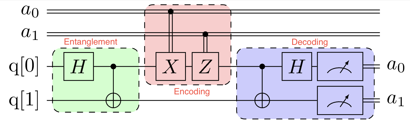
• counterintuitive protocol that allows us to send 2 bits of classical information by sending only 1 qubit, using pre-shared entanglement
• it's often contextualized as a game with Alice and Bob.
• Alice and Bob share and entangled pair of qubits
• Pre-shared Entanglement (Shared Bell pair)
  • $|\Phi^+\rangle = \frac{1}{\sqrt{2}}(|00\rangle + |11\rangle)$
• Alice wants to send 2 bits of classical information (00, 01, 10, or 11) to Bob
  • For 00: Apply Identity $I$ (do nothing)
  • For 01: Apply Pauli-X $X$ (bit flip)
  • For 10: Apply Pauli-Z $Z$ (phase flip)
  • For 11: Apply $XZ$ (bit and phase flip)
• Alice sends her one qubit to Bob (Bob possesses both qubits of the entangled pair)
• Bob decodes the information
  • Inverts the entanglement operation on the two qubits (CNOT followed by Hadamard)
  • Measures each of the qubits
  • The outcome of this measurement reveals the two bits Alice encoded.
• $|\Phi^+\rangle$: is the most common and convenient form (Bell State) of entanglement and is also maximally entangled state despite single-qubit unitary gates.
  • Easy to build circuits for it
  • Symmetric and has nice properties that make it ideal for protocols like superdense coding and teleportation
  • Other Bell states can be generated from $|\Phi^+\rangle$ by applying single-qubit gates.

Superdense Coding Circuit​

• Alice's message $mn$, where each of $m$ and $n$ is a bit (0 or 1)
• Alice's operation can be represented as $Z^m X^n \otimes \mathbb{I} | \Phi^+\rangle$
  • $m=0 \Rightarrow Z^0 = I$ (no phase flip)
  • $m=1 \Rightarrow Z^1 = Z$ (phase flip)
  • $n=0 \Rightarrow X^0 = I$ (no bit flip
  • $n=1 \Rightarrow X^1 = X$ (bit flip)
  • $00 \rightarrow I$
  • $01 \rightarrow X$
  • $10 \rightarrow Z$
  • $11 \rightarrow ZX$
• $Z^m|b\rangle = (-1)^{mb}|b\rangle$ (phase flip)
• $X^n|a\rangle = |a \oplus n\rangle$ (xor operation)

$X^n \left(\frac{1}{\sqrt{2}} (|00\rangle + |11\rangle)\right) = \frac{1}{\sqrt{2}} \left( |n0\rangle + |(1\oplus n)1\rangle \right)$

• $n=0$: $\frac{1}{\sqrt{2}} (|00\rangle + |11\rangle) = |\Phi^+\rangle$
• $n=1$: $\frac{1}{\sqrt{2}} (|10\rangle + |01\rangle)$

$Z^m X^n \left(\frac{1}{\sqrt{2}} (|00\rangle + |11\rangle)\right) = \frac{1}{\sqrt{2}} \left( (-1)^{mn}|n0\rangle + (-1)^{m(1\oplus n)}|(1\oplus n)1\rangle \right)$

• $|n0\rangle$: first qubit is $n$, $(-1)^{mn}$ is the phase factor
• $|(1\oplus n)1\rangle$: first qubit is $1\oplus n$, $(-1)^{m(1\oplus n)}$ is the phase factor
• Bob's decoding operation is the inverse of the entanglement operation
  • $CNOT |a\rangle |b\rangle = |a\rangle |a \oplus b\rangle$

• which is seperable state.
• First qubit is $|n\rangle + (-1)^m|1 \oplus n\rangle$ and second qubit is $|n\rangle$.
• $n, m \in \{0, 1\}$, then apply Hadamard to the first qubit:

• second qubit is $|n\rangle$, so the final state is:

$(-1)^{mn}(-1)^{nm}|m\rangle|n\rangle = |mn\rangle$

Superdense QASM​

OPENQASM 2.0;
qreg q[2];
creg c[2];

// Prepare Bell pair
h q[0];
cx q[0],q[1];

// Alice's encoding
// For message 11: apply X and Z
x q[0];
z q[0];

// Alice sends q[0] to Bob (in simulation, we just proceed)

// Bob's decoding
cx q[0],q[1];
h q[0];

// Measure both qubits
measure q[0] -> c[0];
measure q[1] -> c[1];

QASM Programming​

Custom Gates​

// params: parameters for the gate (e.g., rotation angles)
// q_args: quantum arguments (qubits the gate acts on)
gate NAME(parameters) q_args {
  // Define gate operations
}

gate bell a,b {
  h a;
  cx a,b;
}

qreg q[2];
creg c[2];

// Use the custom bell gate
bell q[0], q[1];

// Measure the qubits
measure q[0] -> c[0];
measure q[1] -> c[1];

Toffoli Gate​

// Toffoli gate (CCX)
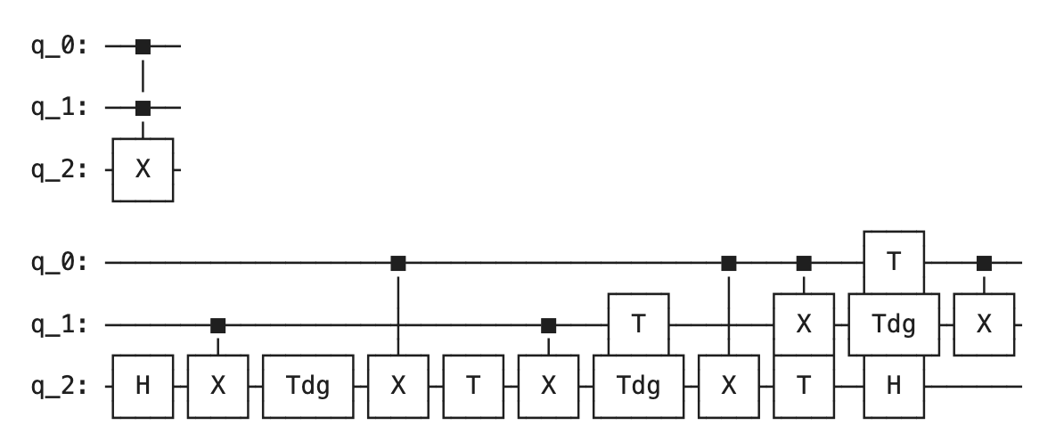
gate ccx a, b, c {
  h c;
  cx b, c;
  tdg c;
  cx a, c;
  t c;
  cx b, c;
  tdg c;
  cx a, c;
  t b;
  t c;
  cx a, b;
  h c;
  t a;
  tdg b;
  cx a, b;
}

Rotation Gates​

// Rotation around Y-axis
gate ry_deg(theta) q {
  ry(theta/180 * pi) q;
}

// Rotation around X-axis
gate rx_deg(theta) q {
  rx(theta/180 * pi) q;
}

Qiskit​

IBM

import qiskit

superdense = qiskit.QuantumCircuit(2, 2)
superdense.draw()

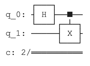
superdense.h(0)
superdense.cx(0, 1)
superdense.draw()

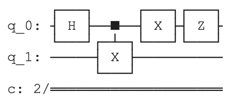
# Alice's encoding for message '11'
superdense.x(0)
superdense.z(0)
superdense.draw()

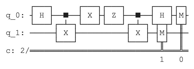
# Bob unentangles the two qubits (reverses the entangling gate)
superdense.cx(0,1)
superdense.h(0)

# The measurement pattern is `measure(qubit to measure, classical bit to store result)`
superdense.measure(0,0)
superdense.measure(1,1)
superdense.draw()

from qiskit.providers.basic_provider import BasicSimulator

sim = BasicSimulator()
# run the circuit on the simulator with 1 shot (execute the circuit once)
result = sim.run(superdense, shots=1).result().get_counts()

print(result)
# {'11': 1}

Custom Gates in Qiskit​

bell = qiskit.QuantumCircuit(2, name='bell')
bell.h(0)
bell.cx(0, 1)
bell_gate = bell.to_gate()

c = qiskit.QuantumCircuit(2)
c.append(bell_gate, [0, 1])
c.draw()

Decompose a custom gate​

ccxgate = qiskit.circuit.library.CCXGate()
ccx = qiskit.QuantumCircuit(3)
ccx.append(ccxgate, [0, 1, 2])

print(ccx)
print(ccx.decompose())

Cirq​

Google

import cirq

alice = cirq.NamedQubit('Alice')
bob = cirq.NamedQubit('Bob')

superdense = cirq.Circuit()
superdense.append([
  cirq.H(alice),
  cirq.CNOT(alice, bob),
])

superdense.append([
  cirq.X(alice),
  cirq.Z(alice),
])

superdense.append([
  cirq.CNOT(alice, bob),
  cirq.H(alice),
])

superdense.append(cirq.measure(alice, bob, key='received'))

print(superdense)

simulator = cirq.Simulator()
result = simulator.run(superdense, repetitions=1)
print(result)
# received=1, 1

Pennylane​

Xanadu

import pennylane as qml

def entangle():
    qml.Hadamard(wires=0)
    qml.CNOT(wires=[0, 1])

print(qml.draw(entangle)())

device = qml.device("default.qubit", wires=[0, 1])

# Wrap the quantum function as a QNode
entangle_qnode = qml.QNode(my_circuit, device)

# Set the number of shots to 10
entangle_qnode = qml.set_shots(entangle_qnode, shots=10)

import numpy as np

state = np.array([1, 1j], dtype=complex)

state = state / np.linalg.norm(state)

def teleport(state):
    # Ensure "state" is loaded into the first qubit
    # (otherwise qubits would start in |0>)
    qml.StatePrep(state, wires=0)

    # Shared entanglement between qubits 1 and 2
    qml.Hadamard(wires=1)
    qml.CNOT(wires=[1, 2])

    # Alice's operation:
    # CNOT from Alice's input qubit to her half of the Bell pair,
    # then Hadamard on the input qubit
    qml.CNOT(wires=[0, 1])
    qml.Hadamard(wires=0)

    # Measurement (store the classical outcomes)
    m0 = qml.measure(0)
    m1 = qml.measure(1)

    # Bob's conditional correction operations
    qml.cond(m1, qml.PauliX)(wires=2)
    qml.cond(m0, qml.PauliZ)(wires=2)

    # Return Bob's qubit as a density matrix
    return qml.density_matrix(wires=2)

print(qml.draw(teleport)(state))

Quantum Teleportation​

• if there is entanglement:
  • we can use it to send 2 bits of classical information by sending 1 qubit (superdense coding)
  • we can use it to send 1 qubit of quantum information by sending 2 bits of classical information (teleportation)
• Alice wants to send a qubit $|\psi\rangle = \alpha|0\rangle + \beta|1\rangle$ to Bob, but only has a classical channel.

Protocol​

1. Alice and Bob share $|\Phi^+\rangle$ (pre-shared entanglement)
2. Alice applies $CNOT$ (her qubit -> her Bell half), then $H$, then measures both, obtaining 2 classical bits (00, 01, 10, or 11)
3. Alice sends $mn$ classically to Bob
4. Bob applies $X^n Z^m$ to his qubit, recovering $|\psi\rangle$

• For 00: Apply Identity $I$ (do nothing)
• For 01: Apply Pauli-X $X$ (bit flip)
• For 10: Apply Pauli-Z $Z$ (phase flip)
• For 11: Apply $XZ$ (bit and phase flip)
• Bob now has a qubit in the state Alice wanted to send $|\psi\rangle$ without Alice ever sending a qubit directly to Bob.

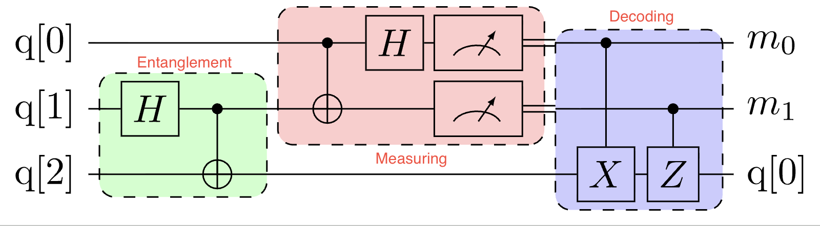
Teleportation Circuit​

$|\psi\rangle \otimes |\Phi^+\rangle = \left(\alpha |0\rangle + \beta |1\rangle\right) \otimes \frac{1}{\sqrt{2}} \left(|00\rangle + |11\rangle\right)$

$|\psi\rangle \otimes |\Phi^+\rangle = \frac{1}{\sqrt{2}} \left(\alpha |0\rangle |00\rangle + \alpha |0\rangle |11\rangle + \beta |1\rangle |00\rangle + \beta |1\rangle |11\rangle\right)$

• Alice applies a $CNOT$ gate with her qubit $|\psi\rangle$ as control and her half of the Bell pair $|\Phi^+\rangle$ as target.
  • $\beta |1\rangle |00\rangle$ becomes $\beta |1\rangle |10\rangle$ (target flips when control is 1)
  • $\beta |1\rangle |11\rangle$ becomes $\beta |1\rangle |01\rangle$ (target flips when control is 1)

$\frac{1}{\sqrt{2}} \Big(\alpha |0\rangle |00\rangle + \alpha |0\rangle |11\rangle + \beta |1\rangle |10\rangle + \beta |1\rangle |01\rangle\Big)$

• Alice then applies a Hadamard gate to her qubit ($|\psi\rangle$).
  • $H|0\rangle = \frac{|0\rangle + |1\rangle}{\sqrt{2}}$
  • $H|1\rangle = \frac{|0\rangle - |1\rangle}{\sqrt{2}}$
• To prepare for measurement, Bell measurement is performed on Alice's two qubits, which can be expressed as:

• Alice measures her two qubits, resulting in one of four possible outcomes corresponding to the classical bits $|mn\rangle$ where $m, n \in \{0, 1\}$
  • Alice's two qubits: $|00\rangle, |0 1\rangle, |1 0\rangle, |1 1\rangle$
  • Bob's qubit is in a state that depends on Alice's measurement outcome

$X^n Z^m |\psi\rangle$

Channels​

• Classical Channel: carries bits (fibre, radio, paper, ...)
• Quantum Channel: carries qubits (can also carry bits)
  • Quantum channels can emulate classical ones, but not vice versa
• Teleportation: classical channel + pre-shared entanglement -> effective quantum channel

Summary​

• In superdense coding, by sending only one qubit and using pre-shared entanglement, Alice can transmit two classical bits of information.
• The operation $X^n \lvert a \rangle = \lvert a \oplus (n \bmod 2) \rangle$ correctly defines the effect of applying the $X$ gate $n$ times.
• The tensor product of two identity operators is the identity operator on the composite space. In symbols, where the subscript is the dimension: $I_2 \otimes I_2 = I_4$.
• The state $\lvert \phi \rangle = \frac{1}{\sqrt{2}}(\lvert 0 \rangle + \lvert 1 \rangle)$ is an eigenstate of the Pauli-$X$ gate with eigenvalue $+1$.
• In the teleportation protocol, the classical communication channel is used to transmit two classical bits from Alice to Bob.
• Three qubits are required for quantum teleportation.
• After the teleportation protocol completes, Bob has a qubit in the state $\lvert \psi \rangle$.
• Of QASM, Qiskit, Cirq, and PennyLane, PennyLane is the only quantum language that spells out the full name of the Hadamard gate for its built-in gates.

Innovation Ecosystem​

• A network of organizations, people and resources that interact with each other to develop and support new ideas, technologies and businesses.
• Innovation Ecosystem
  • Start-up companies
  • Medical Centers
  • Mature Companies
  • City, Regional and State Organizations
  • Providers of Support Services (Legal, Accounting, etc)
  • Venture Capital Funds
  • Colleges & universities

Type of Innovation Ecosystem​

• Corporate innovation ecosystem
• Digital innovation ecosystem
• City-based innovation ecosystem
• High-tech SMEs centered ecosystem (Small and Medium-sized Enterprises)
• University-based ecosystem
• Incubators and Accelerators ecosystems
• Regional and National innovation ecosystems
• Social innovation ecosystems

The core -> New Innovation Initiatives -> Startup Ecosystem -> Customers

Roles and Activites across Innovation Ecosystem​

• Leadership:
  • Ecosystem leader
    • ecosystem governance: decipher roles, coordinate interactions, orchestrate resource flows
    • forging partnerships: attract & link partners, create collaboration, stimulate complementary
    • platform management: build platform, open platform, orchestrate compleentors
    • value management: decipher bases of value, create & capture value
  • Dominator: integrate actors
• Direct Value Creation:
  • Supplier: supply components
  • Assembler: assemble components
  • Complementor: provide complementarities
  • User: define need, provide ideas, purchase & use
• Value Support:
  • Expert: generte knowledge, provide expertise, transfer technology
  • Champion: build connections, provide access to markets
• Entrepreneur Ecosystem:
  • Entrepreneur: co-locate, set-up network
  • Sponsor: give resources, co-develop offering, link to other actors
  • Regulator: provide favorable conditions

Systems Thinking​

• a holistic and non-linear approach to problem solving that focuses on the interactions and patterns within an entire system
• emphasizes relationships and feedback loops instead of analysing individual parts in isolation

Fishbone Diagram​

• common categories to help think broadly about the possible causes include:
• People: skils, training, communication, motivation
• Process / Methods: procedures, or workflows
• Machines / Techonology: tools, equipment, software
• Materials: resources or inputs used
• Environment: workplace or external conditions
• Mangement / Policies: decisions, rules, or leadership

Innovation Networks​

• connected systems of people working together toward shared objectives, often through internal teams and external partners such as suppliers, universities, accelerators, customers, and startups.
• is also part of innovation ecosystem

Types of Innovation Networks​

• Enterpreneur-based
• Internal project teams
• Internal enterpreneur networks
• Communities of practice: can involve players inside and across different organizations
• Spatial clusters: like Silicon Valley, Boston, etc
• Sectoral networks: bring different players together because they share a common sector
• New product or process develoment consortium
• New technology development consortium
• Emerging standards: Exploring and estabilishing standards around innovative technologies
• Supply chain learning
• Learning networks
• Recombinant innovation networks: Cross-sectoral groupings that alloow for networking across boundaries and the transfer of ieads.
• Managed open innovation networks
• User networks
• Innovation markets
• Crowdfunding and new resource approaches

Stakeholder Analysis​

• High power, highly interested people (Engage Closely)
• High power, less interested people (Keep Satisfied)
• Low power, Highly interested people (Keep Informed)
• Low power, less interested people (Monitor)

Tensor Products​

Kronecker product

• a way to multiply vectors and matrices to generate bigger vectors and matrices

$|\psi\rangle \otimes |\phi\rangle = \begin{pmatrix} \psi_0 \\ \psi_1 \end{pmatrix} \otimes \begin{pmatrix} \phi_0 \\ \phi_1 \end{pmatrix} = \begin{pmatrix} \psi_0 \begin{pmatrix} \phi_0 \\ \phi_1 \end{pmatrix} \\ \\ \psi_1 \begin{pmatrix} \phi_0 \\ \phi_1 \end{pmatrix} \end{pmatrix} = \begin{pmatrix} \psi_0 \phi_0 \\ \psi_0 \phi_1 \\ \psi_1 \phi_0 \\ \psi_1 \phi_1 \end{pmatrix}$

$|\psi\rangle \otimes |\phi\rangle \equiv |\psi\rangle |\phi\rangle \equiv|\psi\phi\rangle$

Tensor product of Matrices​

$A \otimes B = \begin{pmatrix} a_{00}B & a_{01}B \\ a_{10}B & a_{11}B \end{pmatrix}$

• The tensor product $|0\rangle \langle1| \otimes |1\rangle \langle0|$ is:

$|0\rangle \langle 1| \otimes |1\rangle \langle 0| = \begin{pmatrix} 0 & 1 \\ 0 & 0 \end{pmatrix} \otimes \begin{pmatrix} 0 & 0 \\ 1 & 0 \end{pmatrix}$

$|0\rangle \langle 1| \otimes |1\rangle \langle 0| = \begin{pmatrix} 0 \cdot \begin{pmatrix} 0 & 0 \\ 1 & 0 \end{pmatrix} & 1 \cdot \begin{pmatrix} 0 & 0 \\ 1 & 0 \end{pmatrix} \\ 0 \cdot \begin{pmatrix} 0 & 0 \\ 1 & 0 \end{pmatrix} & 0 \cdot \begin{pmatrix} 0 & 0 \\ 1 & 0 \end{pmatrix} \end{pmatrix} = \begin{pmatrix} 0 & 0 & 0 & 0 \\ 0 & 0 & 1 & 0 \\ 0 & 0 & 0 & 0 \\ 0 & 0 & 0 & 0 \end{pmatrix}$

• To short hand this, we can write:

$|0\rangle \langle 1| \otimes |1\rangle \langle 0| \equiv |0\rangle|1\rangle \langle 1| \langle 0| \equiv |01\rangle \langle 10|$

• $(|a\rangle \langle b|) \otimes (|c\rangle \langle d|) = (|a\rangle |c\rangle)(\langle b| \langle d|) = |ac\rangle \langle bd|$

Bases​

• The basis for a single qubit is $\{|0\rangle, |1\rangle\}$
• It is given by taking the tensor product of the basis for each qubit:
  • $\{|0\rangle \otimes |0\rangle, |0\rangle \otimes |1\rangle, |1\rangle \otimes |0\rangle, |1\rangle \otimes |1\rangle\}$
  • For short hand, we write $\{|00\rangle, |01\rangle, |10\rangle, |11\rangle\}$
• The computational basis for two qubits is $\{|00\rangle, |01\rangle, |10\rangle, |11\rangle\}$
• For three qubits $\{|000\rangle, |001\rangle, |010\rangle, |011\rangle, |100\rangle, |101\rangle, |110\rangle, |111\rangle\}$

Matrices​

$\{|0\rangle\langle0|,\; |0\rangle\langle1|,\; |1\rangle\langle0|,\; |1\rangle\langle1|\}$

• forms a basis for the space of $2 \times 2$ matrices
• operator basis: a set of matrices that can be used to express any matrix as a linear combination of the basis matrices

$\begin{pmatrix} a & b \\ c & d \end{pmatrix} = a |0\rangle\langle0| + b |0\rangle\langle1| + c |1\rangle\langle0| + d |1\rangle\langle1|$

• One of the basis elements is: $|0\rangle\langle0| \otimes |0\rangle\langle0| = |00\rangle\langle00|$
• Similarly $|0\rangle\langle0| \otimes |0\rangle\langle1| = |00\rangle\langle01|$
• In total, the tensor products yields $4 \times 4 = 16$ basis elements for the space of $4 \times 4$ matrices: $\{|00\rangle\langle00|,\; |00\rangle\langle01|,\; |00\rangle\langle10|,\; |00\rangle\langle11|,\; |01\rangle\langle00|,\; |01\rangle\langle01|,\; \ldots,\; |11\rangle\langle11|\}.$

The Golden Rule of Tensor Products​

What starts on the left of the tensor product says on the left

$(A \otimes B)(|\psi\rangle \otimes |\phi\rangle) = (A|\psi\rangle) \otimes (B|\phi\rangle)$

$(|0\rangle\langle0| \otimes |1\rangle\langle1|)(|00\rangle) \\ = (|0\rangle\langle 0| \otimes |1\rangle\langle1|)(|0\rangle \otimes |0\rangle) \\ \\ = (|0\rangle\langle0||0\rangle) \otimes (|1\rangle\langle1||0\rangle) \\ = |0\rangle \otimes 0 \\ = 0$

• $|\psi\rangle \otimes |\phi\rangle \equiv |\psi\rangle|\phi\rangle \equiv |\psi\phi\rangle$
• $(|\psi\rangle \otimes |\phi\rangle)^\dagger = \langle\psi| \otimes \langle\phi|$
• $(\alpha|\psi\rangle + \beta|\phi\rangle) \otimes |\omega\rangle = \alpha|\psi\rangle \otimes |\omega\rangle + \beta|\phi\rangle \otimes |\omega\rangle$
• $((\langle\psi| \otimes \langle\phi|)(|\omega\rangle \otimes |\eta\rangle)) = \langle\psi|\omega\rangle \langle\phi|\eta\rangle$
• $(A + B) \otimes C = A \otimes C + B \otimes C$
• $A \otimes (B + C) = A \otimes B + A \otimes C$
• $(A \otimes B)(C \otimes D) = AC \otimes BD$
• $(A \otimes B)^\dagger = A^\dagger \otimes B^\dagger$

Entanglement​

• Single-qubit state is a two dimensional vector: $|\psi\rangle = \alpha|0\rangle + \beta|1\rangle$
• where $\alpha$ and $\beta$ are complex numbers such that $\||\psi\rangle\|^2 = |\alpha|^2 + |\beta|^2 = 1$
• Two qubits $\psi_1\rangle$ and $\psi_2\rangle$ can be combined to form a four-dimensional vector: $|\psi_{12}\rangle = |\psi_1\rangle \otimes |\psi_2\rangle \equiv |\psi_1\rangle|\psi_2\rangle \equiv |\psi_1\psi_2\rangle$
• Separable States: can be written as a tensor product of single-qubit states
  • $|\Psi\rangle = \alpha_{00} |00\rangle + \alpha_{01} |01\rangle + \alpha_{10} |10\rangle + \alpha_{11} |11\rangle \\ = |\psi_1\rangle| \otimes \psi_2\rangle$
• if the state is not separable, it is called entangled.
  • entangled: $\frac{1}{\sqrt{2}}(|00\rangle + |11\rangle)$
• if $ad = 0$ and $bc = 0$, then $ac$ or $bd$ must also vanish.
  • separable: $\frac{1}{2}(|00\rangle + |01\rangle) = |0\rangle \otimes \frac{1}{\sqrt{2}}(|0\rangle + |1\rangle)$

Two-Qubit Gates​

• Two-qubit gates are $4 \times 4$ unitary matrices that act on two-qubit states.

CNOT Gate​

Controlled NOT gate

• flips target if control is $|1\rangle$

$\text{CNOT} = \begin{pmatrix} 1 & 0 & 0 & 0 \\ 0 & 1 & 0 & 0 \\ 0 & 0 & 0 & 1 \\ 0 & 0 & 1 & 0 \end{pmatrix} = |0\rangle\langle0| \otimes \mathbb I + |1\rangle\langle1| \otimes X$

SWAP Gate​

• Exchanges the two qubits.

$\text{SWAP} = \begin{pmatrix} 1 & 0 & 0 & 0 \\ 0 & 0 & 1 & 0 \\ 0 & 1 & 0 & 0 \\ 0 & 0 & 0 & 1 \end{pmatrix}$

CZ Gate​

Controlled Z gate

• Applies $Z$ to target if control is $|1\rangle$

$\text{CZ} = \begin{pmatrix} 1 & 0 & 0 & 0 \\ 0 & 1 & 0 & 0 \\ 0 & 0 & 1 & 0 \\ 0 & 0 & 0 & -1 \end{pmatrix}$

Building Multi-Qubit Gates​

• Two qubits $|\psi_1\rangle$ and $|\psi_2\rangle$ can be combined to form a four-dimensional vector:
  • if $U_1$ and $U_2$ are single-qubit gates, then $U_1 \otimes U_2$ is a two-qubit gate that acts on the combined state $|\psi_1\rangle \otimes |\psi_2\rangle$.
  • $(U_1 \otimes U_2)(|\psi_1\rangle \otimes |\psi_2\rangle) = (U_1|\psi_1\rangle) \otimes (U_2|\psi_2\rangle)$
  • For shorthand, $U_1 U_2|\psi_1\psi_2\rangle$

Order of Operations​

• When gates act independently, it doesn't matter the order in which they are apply with the understanding that if only a single gate is applied, identity acts on the other qubits.

$(U_1 \otimes U_2) = (\mathbb I \otimes U_2)(U_1 \otimes \mathbb I) = (U_1 \otimes \mathbb I)(\mathbb I \otimes U_2)$

• Example: Apply $X$ to qubit 1 and $H$ to qubit 2, starting with $|00\rangle$:
• $(X \otimes \mathbb I)|00\rangle = |10\rangle$
• $(\mathbb I \otimes H)|10\rangle \\ = (\mathbb I \otimes H)(|1\rangle \otimes |0\rangle) \\ = |1\rangle \otimes H|0\rangle \\ = |1\rangle \otimes \frac{1}{\sqrt{2}}(|0\rangle + |1\rangle) \\ = \frac{1}{\sqrt{2}}(|1\rangle \otimes |0\rangle + |1\rangle \otimes |1\rangle) \\ = \frac{1}{\sqrt{2}}(|10\rangle + |11\rangle)$

Quantum Circuits​

• A quantum program is a sequance of gates applied to qubits, which are typically assumed to be initialized in the state $|0\rangle$.
• Two qubits start in the state $|0\rangle \otimes |0\rangle = |00\rangle$

$CNOT(H \otimes \mathbb I)|00\rangle = CNOT\left(\frac{1}{\sqrt{2}}(|00\rangle + |10\rangle)\right) = \frac{1}{\sqrt{2}}(|00\rangle + |11\rangle)$

• $S = Ph(\pi/2)$
• $T = Ph(\pi/4)$
• $Z = Ph(\pi)$

Multi-Qubit Gates​

Name	Gates	Matrix
CNOT		$\begin{pmatrix} 1 & 0 & 0 & 0 \\ 0 & 1 & 0 & 0 \\ 0 & 0 & 0 & 1 \\ 0 & 0 & 1 & 0 \end{pmatrix}$
CZ		$\begin{pmatrix} 1 & 0 & 0 & 0 \\ 0 & 1 & 0 & 0 \\ 0 & 0 & 1 & 0 \\ 0 & 0 & 0 & -1 \end{pmatrix}$
SWAP		$\begin{pmatrix} 1 & 0 & 0 & 0 \\ 0 & 0 & 1 & 0 \\ 0 & 1 & 0 & 0 \\ 0 & 0 & 0 & 1 \end{pmatrix}$
Toffoli		$\begin{pmatrix} 1 & 0 & 0 & 0 & 0 & 0 & 0 & 0 \\ 0 & 1 & 0 & 0 & 0 & 0 & 0 & 0 \\ 0 & 0 & 1 & 0 & 0 & 0 & 0 & 0 \\ 0 & 0 & 0 & 1 & 0 & 0 & 0 & 0 \\ 0 & 0 & 0 & 0 & 1 & 0 & 0 & 0 \\ 0 & 0 & 0 & 0 & 0 & 1 & 0 & 0 \\ 0 & 0 & 0 & 0 & 0 & 0 & 0 & 1 \\ 0 & 0 & 0 & 0 & 0 & 0 & 1 & 0 \end{pmatrix}$

• CNOT gate can be $|0\rangle\langle0| \otimes \mathbb I + |1\rangle\langle1| \otimes X$
  • $|0\rangle \text{state} \rightarrow \mathbb I$ (do nothing)
  • $|1\rangle \text{state} \rightarrow X$ (flip the target)
• Larger gates can be built from smaller ones
• Toffoli gate (CCNOT): flips the target if both controls are $|1\rangle$.
• $\text{Toffoli} = |00\rangle\langle00| \otimes \mathbb I_4 + |11\rangle\langle11| \otimes X$
  • two control qubits and one target qubit
  • if both control qubits are $|1\rangle$, then apply $X$
  • $|110\rangle \rightarrow |111\rangle$
  • $|111\rangle \rightarrow |110\rangle$
• Can be generalized to $n$-qubits: $C^{n-1}NOT$ gate, which flips the target if all $n-1$ control qubits are $|1\rangle$.
  • CNOT: $|10\rangle \rightarrow |11\rangle$ and $|11\rangle \rightarrow |10\rangle$
  • Toffoli: $|110\rangle \rightarrow |111\rangle$ and $|111\rangle \rightarrow |110\rangle$
  • 3-control gate: $|1110\rangle \rightarrow |1111\rangle$ and $|1111\rangle \rightarrow |1110\rangle$

$(\mathbb I - |111\ldots\rangle\langle 111\ldots|)\otimes \mathbb I + |111\ldots\rangle\langle 111\ldots|\otimes U$

The Rules of Quantum Computing​

Initialization​

• An $n$-qubit computation starts in the all-zero state:

$|phi\rangle = |0\rangle \otimes |0\rangle \otimes \ldots \otimes |0\rangle = |00\ldots0\rangle$

Algorithm​

• Apply a sequence of unitary gates to obtain the final state:

$U = U_1U_2\ldots U_m \implies U|\psi\rangle$

Measurement​

The Born Rule

• Reading $n$ qubits producs $n$ classical bits.
• The probability of outcome $b_1b_2\ldots b_n$:

$Pr(b_1b_2\ldots b_n) = |\langle b_1b_2\ldots b_n|\psi\rangle|^2$

• $|\psi\rangle$: initial state of the system
• $U$: an unitary matrix summing up the gates applied to the system
• $U|\psi\rangle$: final state of the system
• $\langle b_1b_2\ldots b_n|U|\psi\rangle$: the amplitude of the outcome $b_1b_2\ldots b_n$
• $|\text{amplitude}|^2$: The probability of the outcome $b_1b_2\ldots b_n$ being observed when measuring the system
  • if $\frac{1}{\sqrt{2}}(|00\rangle + |11\rangle)$
  • then $Pr(00) = Pr(11) = \frac{1}{2}$

Post-measurement States​

Measurement causes the state to collapse

• Measuring all qubits: outcome $b_1 \ldots b_n$ collapses state to $|b_1 \ldots b_n\rangle$
• Measuring a subset: keep matching terms and renormalize.

$|\psi\rangle = c_{00\ldots0}|00\ldots0\rangle + c_{00\ldots1}|00\ldots1\rangle + \ldots + c_{11\ldots1}|11\ldots1\rangle$

• If we measure all qubits, we get outcome $b_1b_2\ldots b_n$
  • The state will collapse to $|\psi'\rangle = |b_1b_2\ldots b_n\rangle$
  • The probability of this outcome is $Pr(b_1b_2\ldots b_n) = |\langle b_1b_2\ldots b_n|\psi\rangle|^2$

$|\psi\rangle = \alpha|00\rangle + \beta|01\rangle + \gamma|10\rangle + \delta|11\rangle$

• If we measure only the first qubit, and get outcome $0$, the state maintains only terms with $0$ in the first position:
  • $|00\rangle$ and $|01\rangle$
  • The remaining state is $|\psi'\rangle = \alpha|00\rangle + \beta|01\rangle$
  • $|10\rangle$ and $|11\rangle$ are removed from the state
• This gives us the unnormalized state: $|\psi'\rangle_{unnorm} = \alpha|00\rangle + \beta|01\rangle$
• The probability of this outcome is $Pr(0) = |\alpha|^2 + |\beta|^2$
  • $|00\rangle$ and $|01\rangle$ are the only terms that contribute to the probability of outcome $0$ for the first qubit
• After measurement, the state must be $\||\psi\|^2 = 1$, so we need to renormalize the state:

$|\psi'\rangle = \frac{(\alpha|00\rangle + \beta|01\rangle)}{\sqrt{|\alpha|^2 + |\beta|^2}}$

QASM2.0​

Image Gradient​

• It is a directional change in the intensity or color in an image.
• can be used to extract valuable information from images.
• commonly used in edge detection.
• ➡️ Change is X-directions, ⬇️ Change is Y-directions.
• Combining both X and Y diretion to estimate if changes are in both directions.

HoG, Histogram of Oriented Gradient​

To find edge and shape of the object in the image

• Computing Image Gradient
  • Use the horizontal and vertical filters to compute gradient values
• Compute the strength/magnitude and direction of gradient
  • Strength/Magnitude(g): $\sqrt{g_x^2 + g_y^2}$
  • Direction($\theta$): $\tan^{-1}(g_y / g_x)$
• Create orientation histogram
  • Divide the image into small connected regions called Cells which is a 8x8 patch
  • Create cell histogram based on gradient direction and magnitude
  • 64 (8x8) gradient vectors are put into a 9-bin histogram.
  • The bins are the gradient directions ($\theta$) quantized into 9-bins
• Block Normalization
  • 16x16 pixels blocks or 22 cells are used for normalization, which has 4 histograms.
  • Normalization will make it scale/multiplication invariant
  • Each block will represent 36x1 element vector
• Intensity: brightness of the pixel
• Saturation: HSV color space, the amount of gray in the color
• Calculate the HoG feature vector
  • Each of the 36x1 vectors in each blocks are concatenated into one big vector
  • Size of the vector will be 36xN, where N is the number of blocks in the image
• Hog feature extractor