RL 011

Model Based RL

• Model: Transition Probability, Reward Function, State, Action, Discount Factor
• Planning: use the learned models to evaluate possible actions, construct or iprove a value function or policy using Value/Policy Iteration.
• Underlying MDP: The env's actual state transitions and reward structure.
  • Transition Model $P(s'|s,a)$
  • Reward Model $R(s,a)$
  • Goal: Approximate the env's MDP and use if for planning.

Aspect	Model-Free RL	Model-Based RL
Environment Model	No model available (transition dynamics)	Learn a model from experience
Learning	Directly learn a value function and/or policy from experience	Use the learned model to plan a value function and/or policy
Methods	Learn directly from experience	Use a simulator with DP, Model-Free RL, or Policy Search

Advantages of Model-Based RL

• Efficient Model Learning: Supervised learning can efficiently learn transition and reward models from experience.
• Model Uncertainty: The learned model can estimate uncertainty in its prediction

Disadvantages of Model-Based RL

• Two-Step Process: First learn the environment model, then use it to construct a value function or policy.
• Two Sources of Approximation Error:
  • Approximated Model Error: The learned model may inaccurately predict transitions or rewards.
  • Approximated Planning Error: Planning with the learned model may produce approximate or suboptimal results.
  • Compounding Error: Model and planning errors can accumulate, reducing the accuracy of the final policy.

MDP Model

$\text{MDP} = \langle S, A, P, R \rangle_{\eta}$

• Assumption: State space $S$ and Action space $A$ are known and the env satisfies the Markov property.
• Model $\mu = \langle P_{\eta}, R_{\eta} \rangle$ is parameterized by $\eta$ and represents state-transitions and rewards.
  • $P_{\eta} \approx P$
  • $R_{\eta} \approx R$

$S_{t+1} \sim P_{\eta}(s_{t+1} | s_t, a_t)$ $R_{t+1} \sim R_{\eta}(r_{t+1} | s_t, a_t)$

$P(s_{t+1}, R_{t+1} | s_t, a_t) = P(s_{t+1} | s_t, a_t) P(R_{t+1} | s_t, a_t)$

• Assume that the next state and reward are conditionally independent given the current state and action (not a consequence of the Markov property).
• This allows transition and reward distributions to be modeled separately.

Model Learning

• Goal: Approximate a model $\mu_\eta$ from experience $\{S_1, A_1, R_2, \ldots, S_T\}$.
• Supervised Learning: Use $(S_t, A_t)$ as input and $(R_{t+1}, S_{t+1})$ as targets.
• Loss Function: Measure prediction errors using a loss function (e.g., MSE).
• Empirical Loss: Average prediction error over observed training data.
• Use supervised learning framework, find parameters $\eta$ that minimize empirical loss (MSE).

$$\eta^* = \arg \min_\eta L(\eta)$$

Lookup Table Model

• Underlying Model is presented as a lookup table.
• A model is an explicit $\text{MDP}, \hat{P}, \hat{R}$

$\hat{P}_{ss'}^a = \frac{1}{N(s,a)} \sum_{t=1}^T 1((S_t, A_t, S_{t+1}) = (s,a,s'))$

• $N(s,a)$ is the number of times State-Action pair has been visited.
• $1$: Indicator function that is 1 if the condition is true, 0 otherwise.
• $\hat{P}_{ss'}^a$ is the estimated probability of transitioning from state $s$ to state $s'$ under action $a$.

$\hat{P}(s'|s,a) = \frac{N(s,a,s')}{N(s,a)}$

• Estimated Transition Probability by counting the number of times the State-Action-Next State tuple has been observed.

$$\hat{R}_s^a = \frac{1}{N(s,a)} \sum_{t=1}^T 1((S_t, A_t) = (s,a)) R_{t+1}$$

• Calculate the average reward for the State-Action pair.

Single Action MRP Example

Two States $\{A, B\}$ and no discount, 8 episodes of learning.

• A → B: 100% transition probability, reward = 0.
• B → Terminal: 75% chance of reward 1, 25% chance of reward 0.

Episode	Experience
1	A, 0, B, 0
2	B, 1
3	B, 1
4	B, 1
5	B, 1
6	B, 1
7	B, 1
8	B, 0

• MC: Estimates values using observed complete returns.
  • $V(B) = 6/8 = 0.75$
  • $V(A) = 0$
• TD: Uses bootstrapping, updates a state's value using the estimated value of the next state.
  • $V(B) = 0.75$
  • $V(A) \leftarrow \gamma + \gamma V(B) = 0 + 0.75 = 0.75$
  • Requires a backup of $A$ after $V(B)$ has been learned.

Planning with a model

• Given Model $\mu_\eta = \langle P_{\eta}, R_{\eta} \rangle$
• Solve $\text{MDP} \langle S, A, P_{\eta}, R_{\eta} \rangle$ by $\eta$.
• With Planning algorithm:
  • Value Iteration
  • Policy Iteration
  • Tree searching
  • etc.

Sample-based Planning

• Generate a lot of samples or data then, use model free methods such as MC, SARSA, Q-learning, etc. to plan.
• $S_{t+1} \sim P_{\eta}(S_{t+1} | S_t, A_t)$
• $R_{t+1} \sim R_{\eta}(R_{t+1} | S_t, A_t)$
• Data Efficiency: Reduce real environment interactions by learning from simulated experiences.

Monte Carlo Search

• Given a model $\mu_v$ and simulated policy $\pi$
• For each $a \in A$:

$$Q(S_t, a) = \frac{1}{K} \sum_{k=1}^K G_t$$

• Simulate $k$ episodes from current state $s_t: \{ s_t, a, R_{t+1}^k, \ldots, S_T^k \} \sim \mu_v, \pi$
• Evaluate actions by mean returns (MC evaluation)
• $G_t^{(k)}$: Return from the $k$-th simulation.
• Select current action with max value

$a_t = \arg\max_{a \in A} Q(s_t, a)$

e.g.

Action	Episode 1	Episode 2	Episode 3
Left	3	5	4
Right	2	1	3

• $Q(s_t, \text{Left}) = \frac{3 + 5 + 4}{3} = 4$
• $Q(s_t, \text{Right}) = \frac{2 + 1 + 3}{3} = 2$
• Select action with max value: $\text{Left}$

Expectimax Tree

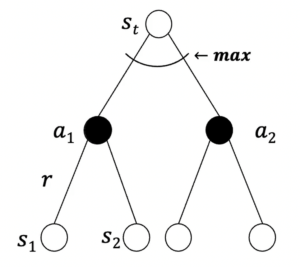
• White Node: Choose action with max value.
• Black Node: Average state values of all possible actions.
• Compute Optimal $Q(s,a)$ values for the current state by construction an expectimax tree.

$$Q(s,a)=\sum_{s'}P_\nu(s'|s,a) \left[R_\nu(s,a,s')+\gamma V(s')\right]$$ $$V(s)=\max_a Q(s,a)$$

• $P_\nu(s'|s,a)$: Transition probability.
• $R_\nu(s,a,s')$: Expected Reward
• $V(s')$: Value of the next state.

Limitations of Expectimax Tree

$$O((|\mathcal S|\times|\mathcal A|)^H)$$

• Scaling Exponentially with Depth: Tree size grows exponentially with depth $H$.
• $|\mathcal S|$: Number of possible states.
• $|\mathcal A|$: Number of possible actions.
• $H$: Depth of the tree.

Monte Carlo Search Tree, MCTS

• Given a model $\mu_v$
• Build a search tree rooted at the current state $s_t$, sample actions and next states.
• Iteratively Construct and update the tree by performing $K$ simulation episodes starting from the root node.
• Once search is finished, select the current action with maximum value in the search tree.

$a_t = \arg\max_{a \in A} Q(s_t, a)$