RL 006

Known MDP vs Unknown MDP

Aspect	Known MDP	Unknown MDP
Environment Knowledge ($P, R$)	Full knowledge of state transition dynamics $P$ and reward function $R$	$P$ and $R$ are unknown; agent must explore the environment
Problem Approach	Well-defined optimization problem $\rightarrow$ Pure planning via computation	Trial-and-error interaction $\rightarrow$ Must learn and optimize simultaneously
Primary Goal	Directly compute the optimal policy ($\pi_*$)	Learn and optimize policies without prior model knowledge
Representative Methods	Value Iteration, Policy Iteration (Dynamic Programming)	Monte Carlo, Q-Learning, SARSA (Reinforcement Learning)
Paradigm	Model-based (Planning)	Model-free (Reinforcement Learning)

Model-based vs Model-free

Aspect	Model-Based Learning	Model-Free Learning
Model Access ($P, R$)	Has full access to transition dynamics $P$ and reward function $R$	No access to environment dynamics ($P$ and $R$ are unknown)
Optimization Approach	Direct mathematical computation and planning using the known model	Direct learning and trial-and-error optimization through interaction
Estimation Source	Computes values and optimal policy $\pi_*$ via dynamic programming equations	Estimates $v_\pi, q_\pi$, and $\pi_*$ directly from sampled experience
Computation vs. Sampling	Pure computation / Planning (requires no real-time environment sampling)	Sample-based learning (requires trajectories / episodic experience)
Typical Methods	Policy Iteration, Value Iteration (DP)	Monte Carlo Methods, TD Learning, Q-Learning, SARSA

Monte Carlo Methods

• A Computational technique that uses random sampling and statistical methods to solve complex problems and estimate numerical results.
  • Named after the Monte Carlo Casino in Monaco.
  • It means Estimate an unknown quantity by sampling, and averaging what you observe.
• Used fo any estimation method whose operation involves a significant random component.
• Used in mathematics, physics, engineering, finance, computer science, etc.
• It is particularly valuable when an analytical solution is difficult or impossible to obtain.

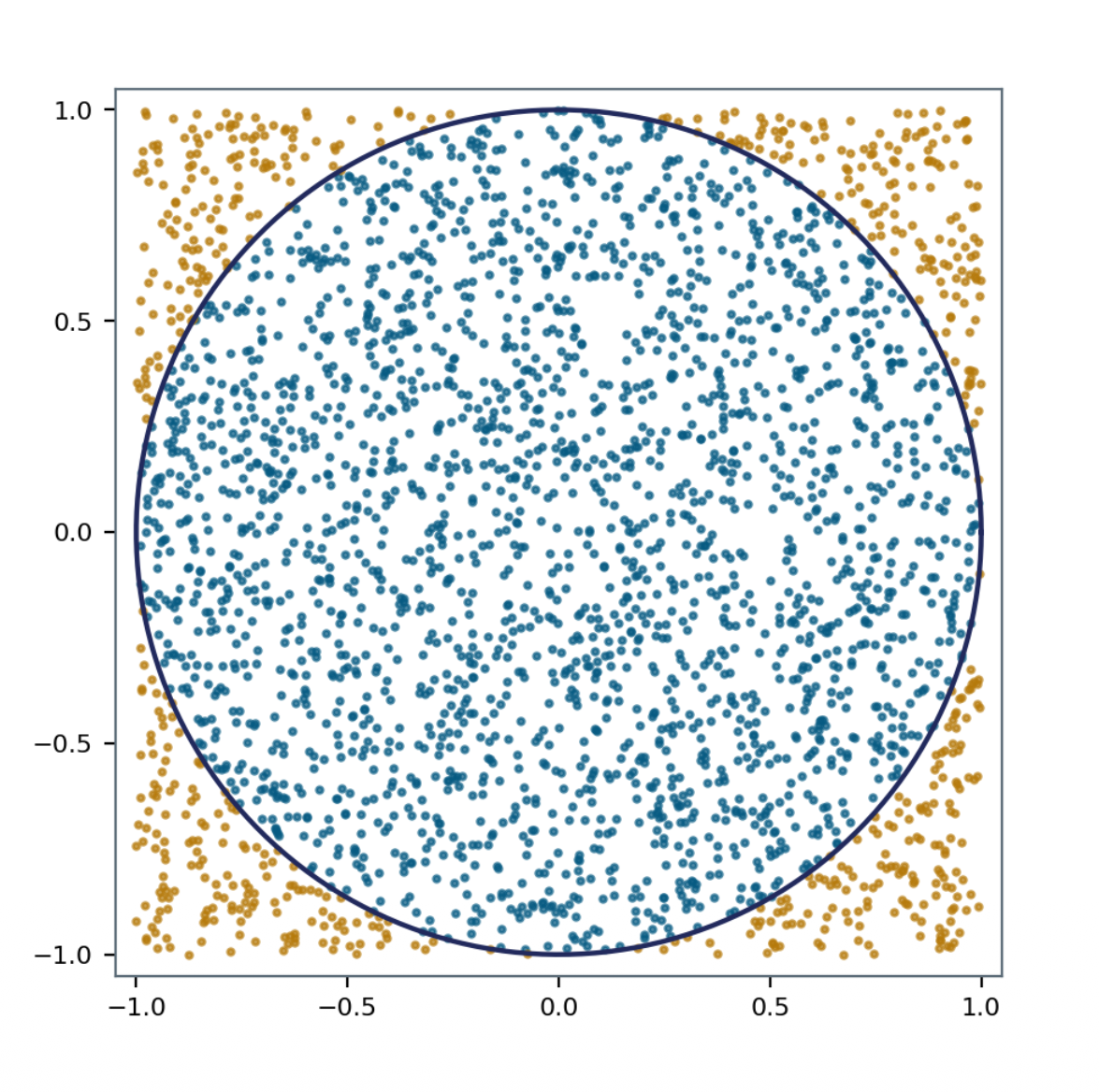
Estimating $\pi$ by Sampling (Monte Carlo Simulation)

• Mechanism:
  • Generate uniform random points $(x, y) \in [-1, 1] \times [-1, 1]$.
  • Count points falling inside the unit circle ($x^2 + y^2 \le 1$).
  • Estimate $\pi$ via area proportions:

$$\begin{aligned} \frac{\text{Area}_{circle}}{\text{Area}_{square}} = \frac{\pi}{4} \\ & \pi \approx 4 \times \frac{\text{\#points inside circle}}{\text{\#total points}} \end{aligned}$$

• Empirical Validation:
  • Total samples ($n$): $3000$ points
  • Estimated value: $\pi = 3.1386666666666665$
  • Relative error: $-0.0931\%$ from true value ($\approx 3.14159265$)

Monte Carlo Prediction

$v_\pi(s) = \mathbb{E}_{\pi}[G_t | S_t = s] \approx \frac{1}{N} \sum_{i=1}^{N(s)} G^{(i)}$

• $\frac{1}{N} \sum_{i=1}^{N(s)} G^{(i)}$: Mean of the returns/rewards
• Model-Free Learning: Operates without prior knowledge of transition dynamics $P$ or reward function $R$.
• Learning from Complete Episodes: Learns state-value functions $v_\pi$ exclusively from full trajectories under policy $\pi$. Only works for episodic tasks where termination at step $T$ is guaranteed.
• No Bootstrapping: Does not update estimates using other value estimates $v(s')$; instead, updates rely solely on actual empirical returns observed at the end of the episode.
• Empirical Mean Returns: The value of state $s$ is estimated by the sample average of all observed returns starting from $s$:

An Episode of Experience & Return Formulation

• Trajectory Structure: $S_0 \xrightarrow{A_0, R_1} S_1 \xrightarrow{A_1, R_2} S_2 \dots \xrightarrow{A_{T-1}, R_T} S_T$
• Discounted Return ($G_t$): $G_t = R_{t+1} + \gamma R_{t+2} + \gamma^2 R_{t+3} + \dots + \gamma^{T-t-1} R_T$
• Discount Factor ($\gamma = 1$): For episodic tasks with terminal-only rewards (such as Blackjack), setting $\gamma = 1$ is standard practice because the episode length is finite.

First-Visit Monte Carlo

• First-Visit MC estimates the value function $V(s)$ by averaging returns following only the first occurrence of state $s$ within each sampled episode.
• Algorithmic Flow:
  • Initialize counters $N(s) \leftarrow 0$ and accumulate returns: $G(s) \leftarrow 0 \quad \forall s \in S$
  • Sample a complete episode $i = \{S_{i,0}, A_{i,1}, R_{i,2}, \dots, S_{i,T_i}\}$ generated under policy $\pi$
  • Compute return $G_{i,t} = \sum_{k=t+1}^{T_i} \gamma^{k-t-1} R_{i,k}$ from step $t$ to termination.
  • Only for the first time step $t$ where state $s$ appears in episode $i$:
    • $N(s) \leftarrow N(s) + 1$ (Increment counter for total first visits)
    • $G(s) \leftarrow G(s) + G_{i,t}$ (Increment total return)
    • $V(s) \leftarrow \frac{G(s)}{N(s)}$ (Update the value by mean return)

$A \xrightarrow{R_1=1} B \xrightarrow{R_2=2} A \xrightarrow{R_3 = 1} C \xrightarrow{R_4 = 1} \text{terminal}$

State s	$N(s)$	$G(s)$	$V(s) = \frac{G(s)}{N(s)}$
A	1	9	9.00
B	1	8	8.00
C	1	5	5.00

Every-Visit Monte Carlo

• Every-Visit MC treats every single occurrence of state $s$ within an episode as a valid data sample, accumulating its corresponding return into the empirical mean.
• Algorithmic Flow:
  • Initialize counters $N(s) \leftarrow 0$ and accumulate returns: $G(s) \leftarrow 0 \quad \forall s \in S$
  • Sample a complete episode $i = \{S_{i,0}, A_{i,1}, R_{i,2}, \dots, S_{i,T_i}\}$ generated under policy $\pi$
  • Compute return $G_{i,t} = \sum_{k=t+1}^{T_i} \gamma^{k-t-1} R_{i,k}$ from step $t$ to termination.
  • For each time step $t$ where state $s$ appears in episode $i$:
    • $N(s) \leftarrow N(s) + 1$ (Increment counter for total visits)
    • $G(s) \leftarrow G(s) + G_{i,t}$ (Increment total return)
    • $V(s) \leftarrow \frac{G(s)}{N(s)}$ (Update the value by mean return)

$A \xrightarrow{R_1=1} B \xrightarrow{R_2=2} A \xrightarrow{R_3 = 1} C \xrightarrow{R_4 = 1} \text{terminal}$

State s	$N(s)$	$G(s)$	$V(s) = \frac{G(s)}{N(s)}$
A	2	9+6=15	7.50
B	1	8	8.00
C	1	5	5.00

Dimension	First-Visit MC	Every-Visit MC
Returns used per episode	Only the first occurrence	Every occurrence
Sample independence	Independent across episodes (i.i.d.)	Correlated within an episode (mitigated by sampling)
Bias (finite samples)	Unbiased	Biased, but $\text{bias} \to 0$
Convergence	Consistent (Law of Large Numbers)	Consistent (as $\text{episodes} \to \infty$)
Implementation	Requires a "seen this episode?" check	Simpler — no check needed
Practical Use	Standard theoretical baseline	Frequently preferred (uses all available data)

Incremental Mean

$\mu_k = \frac{1}{k} \sum_{j=1}^{k} x_j$

$$\begin{aligned} \mu_{k+1} &= \frac{1}{k+1} \sum_{j=1}^{k+1} x_j \\ &= \frac{1}{k+1} \left( \sum_{j=1}^{k} x_j + x_{k+1} \right) \\ &= \frac{1}{k+1} \left( k \mu_k + x_{k+1} \right) \\ &= \mu_k + \frac{1}{k+1} (x_{k+1} - \mu_k) \end{aligned}$$

• New estimate = Old estimate + step-size * (new sample - old estimate).
• Memory efficient: Only need to store the old estimate ($\mu_k$) and the number of visits ($k$).

Incremental Monte Carlo

• Updates the value function $V(s)$ incrementally after each trajectory without requiring memory to store individual past returns.
• Algorithmic Flow:
  • Initialize $N(s) \leftarrow 0$ and $V(s) \leftarrow 0$ for all $s \in S$.
  • Episode sampling: Execute episode $i$ under policy $\pi$ and compute returns $G_{i,t} = \sum_{k=t+1}^{T_i} \gamma^{k-t-1} R_{k}$.
  • Incremental update: For each visited state $s$ at time step $t$:
    • $N(s) \leftarrow N(s) + 1$ (Increment counter for total visits)
    • $V(s) \leftarrow V(s) + \alpha (G_{i,t} - V(s))$ (Update the value by mean return)
    • Where $G_{i,t} - V(s)$ represents the temporal difference (TD) error between the sampled return target and the current estimate.
• Choice step size $\alpha$
  • $\alpha = \frac{1}{N(s)}$: Replicates the exact empirical sample-average of Every-Visit MC where all observed samples receive equal weight.
  • $\alpha = \text{constant}$: Implements an exponential recency-weighted running average that decays outdated experience, making it suited for non-stationary environments where MDP dynamics change over time.
• Cons:
  • Requires a significant number of episodes to converge to the true value function.
  • Requires to terminate the episode.

Model-free Control

• The MDP model is unknown, or too large/complex to use directly.
• But experience can be sampled.
• Applications:
  • Robo soccer
  • Autonomous vehicles
  • Robotics
  • Game playing
  • Recommender systems
  • Finance & portfolio management

On-Policy vs Off-Policy

Dimension	On-Policy Learning	Off-Policy Learning
Definition	Evaluates and improves the exact same policy currently used to generate action decisions	Evaluates/improves a target policy ($\pi$) while behaving via a different behavior policy ($b$)
Data Generation	Trajectories must be generated by the current active policy $\pi$	Trajectories can come from exploratory policies, historical logs, or human demonstrations
Exploration Trade-off	Must balance exploration directly within the target policy (e.g., $\epsilon$-greedy)	Separates exploration (behavior policy) from exploitation/optimality (target policy)
Representative Algorithms	GLIE Monte Carlo Control, SARSA	Q-Learning, Deep Q-Networks (DQN)

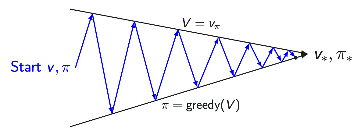
General Policy Iteration

• Alternates between Policy Evaluation ($V \approx v_\pi$ or $Q \approx q_\pi$) and Policy Improvement ($\pi \leftarrow \text{greedy}$).
• This interplay drives the system asymptotically toward the optimal pair $(v_*, \pi_*)$ or $(q_*, \pi_*)$.

$\pi'(s) = \text{argmax}_{a \in A} \big( \mathcal{R}(s, a) + \gamma \sum_{s' \in S} \mathcal{P}(s' | s, a) V(s') \big)$

• Why $V(s)$ Fails in Model-Free Settings:
  • Finding the maximizing action over $V(s)$ strictly requires the transition model $P(s' \mid s, a)$ and reward function $R(s, a)$.
  • In Model-Free RL, these dynamics are unavailable; hence, $V(s)$ alone cannot guide policy updates without an explicit environment model.

$\pi'(s) = \text{argmax}_{a \in A}Q(s,a)$

• Model-Free Advantage:
  • By estimating $Q(s, a)$ directly through sample episodes, policy improvement requires no knowledge of $P$ or $R$.
  • This fundamental shift makes $Q(s, a)$ estimation the standard paradigm for Model-Free Control (Monte Carlo Control, SARSA, Q-Learning).

	$V(s)$	$Q(s, a)$
Question	How good is this state?	How good is this action in this state?
Includes Action?	No	Yes
Policy Evaluation	Very suitable	Slightly more difficult
Policy Improvement	Requires a model	Directly possible
Model-Free Control	Inconvenient	Very suitable

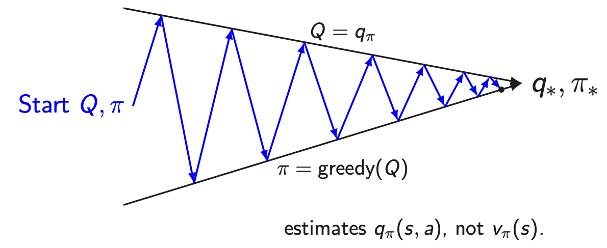
• This is why MC Control estimates $q_\pi(s,a)$, not $v_\pi(s)$.

Exploration Problem

$$a = \arg\max_a Q(s,a)$$

• A greedy agent always chooses the action with the highest current estimated value.
• But what if the current $Q(s,a)$ estimates are inaccurate?

Mystery Box Example

Initially,

$$Q(\text{red}) = 0, \qquad Q(\text{blue}) = 0$$

1. Open the red box:
   $R = 0 \rightarrow Q(\text{red}) = 0$

2. Open the blue box:
   $R = +1 \rightarrow Q(\text{blue}) = 1$

3. Keep opening the blue box:
   $R = +1, +3, +2, \ldots \rightarrow Q(\text{blue}) \approx 2$

4. A purely greedy agent now keeps choosing the blue box because
   $Q(\text{blue}) > Q(\text{red})$.

5. However, the red box may actually be better. For example,
   $\mathbb{E}[R \mid \text{red}] = 5$.

   The agent does not know this because it sampled the red box only once.

Exploitation vs. Exploration

• Exploitation: Choose the action that currently has the highest estimated value.
• Exploration: Try less-sampled or unfamiliar actions to discover whether they may actually be better.
• In this example, the agent should occasionally explore the red box because it has not been sampled enough to confidently conclude that it is worse.

$\epsilon$-Greedy Exploration

$$\pi(a|s) = \begin{cases} \text{greedy action \quad with high probability} \\ \text{random action \quad with probability $\epsilon$} \\ \end{cases}$$

• if $\epsilon = 0.1$, then the agent will choose the greedy action with probability $0.9$ (Exploitation)
• And the random action with probability $0.1$ (Exploration).
• Policy Improvement Theorem:
  • for any $\epsilon$-greedy policy $\pi$
  • The $\epsilon$-greedy policy $\pi'$ is as good or better than the original policy $\pi$: $v_{\pi'}(s) \geq v_{\pi}(s)$

Monte Carlo Control

• Traditional Policy Iteration:
  • Fix the policy $\pi$.
  • Evaluate the current policy until $Q$ is sufficiently close to $q_\pi(s,a)$.
  • Improve the policy using the estimated action values.
  • Repeat policy evaluation and policy improvement.
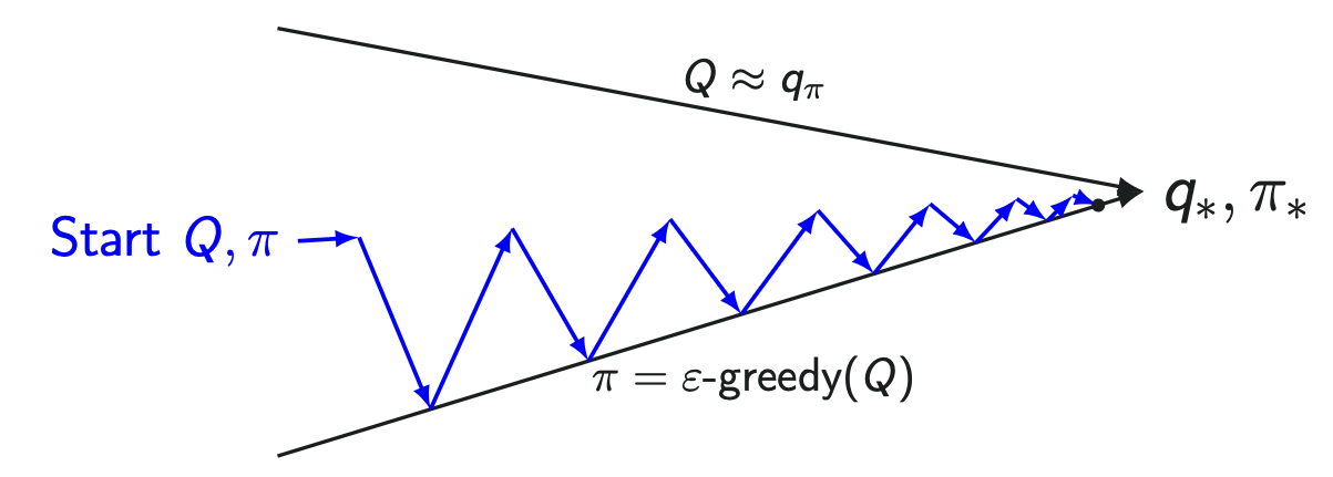
• Monte Carlo Control:
  • Perform MC Policy Evaluation after every episode.
  • Improve the policy using $\epsilon$-greedy after every episode.
  • $Q_1 \rightarrow \pi_1 = \epsilon\text{-greedy}(Q_1)$
  • $Q_2 \rightarrow \pi_2 = \epsilon\text{-greedy}(Q_2)$
  • $\cdots$
  • Eventually approaches $(q_*, \pi_*)$ under appropriate convergence conditions.

$$\text{Evaluate a little} \rightarrow \text{Improve} \rightarrow \text{Evaluate a little} \rightarrow \text{Improve} \rightarrow \cdots$$

GLIE

Greedy in the Limit with Infinite Exploration

1. $\lim_{k \to \infty} N_k(s,a) = \infty$
2. $\lim_{k \to \infty} \pi_k(a|s) = 1(a = \argmax_{a' \in A} Q_k(s,a'))$

• Explore enough early -> Explore less over time -> Eventually greedy.
  • $N_k(s,a)$: How many times the state-action pair $(s,a)$ has been visited in the $k$-th episode.
  • $\pi_k \rightarrow \text{greedy}(Q_k)$
• Infinite exploration first, greedy behavior in the limit.

GILE Monte Carlo Control

• Algorithm flow:
  • Run episode $k = \{S_0, A_0, R_1, \dots, S_{T}\}$ with policy $\pi_k$.
  • For each state-action pair $(s,a)$ in the episode:
    • $N_k(s,a) \leftarrow N_k(s,a) + 1$
    • $Q_k(s,a) \leftarrow Q_k(s,a) + \frac{1}{N_k(s,a)} (G_k - Q_k(s,a))$
  • Improve the policy based on the new $Q$ value.
    • $\epsilon \leftarrow \frac{1}{k}$
    • $\pi \leftarrow \epsilon\text{-greedy}(Q)$
  • Repeat until convergence.
• old estimate + step-size * (new sample - old estimate).
  • old estimate = $Q(S_t, A_t)$
  • new sample = $G_t$
  • step-size = $\frac{1}{N_k(s,a)}$
• Run Episode → Update Q → Reduce $\epsilon$ → Improve Policy

DP vs MC

• Dynamic Programming:
  • Model-based
  • Bootstrapping: Updating a value estimate using another estimated value instead of waiting for the final outcome.
  • Lower variance
• Monte Carlo:
  • Model-free
  • No bootstrapping: It uses rewards that actually occurred, not an estimated value of the next state.
  • Uses complete sampled returns
  • Requires episodic tasks
  • Higher variance