RL 007

Temporal-Difference Learning

Updates a guess towards a guess.

• Model-free: No MDP Dynamics or Rewards
• Learns directly from episodes of experience.
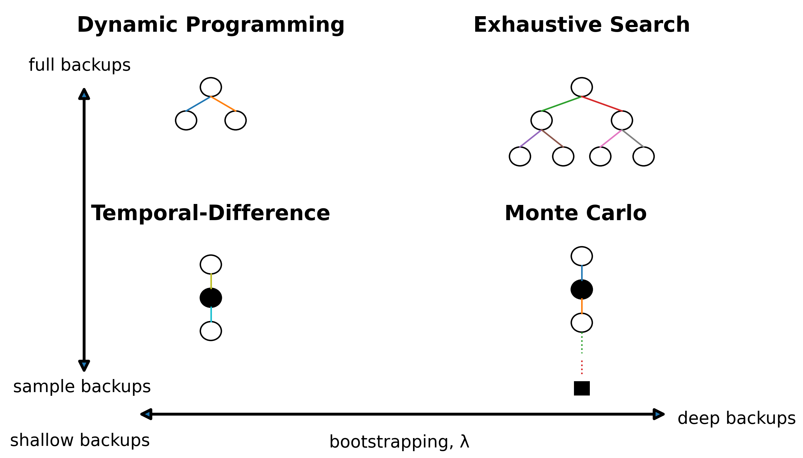
• Bootstrapping: Estimate value function using estimated value from incomplete episodes.
  • Update estimate using another estimate.
• Updates the estimate of $V$ immediately after each step.
• Combines Monte Carlo and Dynamic Programming (Bootstrapping idea).

MC

$V(S_t) = V(S_t) + \alpha [\underbrace{G_t}_{\text{Goal}} - \underbrace{V(S_t)}_{\text{Previous estimate}} ]$

• Update $V(S_t)$ towards the actual return.
• $\alpha = \frac{1}{n}$: Every-visit MC.
  • gives equal weight to all past samples in the arithmetic mean.
• Fixed $\alpha > \frac{1}{n}$: gives more weight to recent experience and reduces the influence of older episodes faster.
  • $\alpha = 0.1, \quad V(S) = 10$
  • $V(S) \leftarrow 10 + 0.1 (20 - 10) = 11$
  • $V(S) \leftarrow 11 + 0.1 (30 - 11) = 12.9$
  • Move 10% of the way towards the new value.

One-Step Bootstrapping

$\text{TD}(0) \rightarrow \text{TD}(\lambda) \rightarrow \text{TD}(1) \approx \text{MC}$

• $\lambda$ controls how much longer-term return information is used in the TD update.
  • It controls how far into the future TD learns from.
• $\lambda = 0$: uses one-step bootstrapping, corresponding to TD(0).
• As $\lambda$ increases, rewards further into the future have more influence on the update.
• $\lambda = 1$: approaches the Monte Carlo return in episodic tasks.

$V(S_t) = V(S_t) + \alpha [\underbrace{\underbrace{R_{t+1} + \gamma V(S_{t+1})}_{\text{TD target}} - V(S_t)}_{\text{TD Error}} ]$

• Only one immediate reward is used $R_{t+1}$.
• Everything after that is replaced by the current guess $V(S_{t+1})$ instead of actual future rewards.
• It uses actual reward for the first step and the estimated value/guess for the rest.

MC
Sₜ ──Rₜ₊₁──> Sₜ₊₁ ──Rₜ₊₂──> ... ──> Terminal
│                                        │
└────────── episode 끝까지 기다림 ────────┘
                   ↓
               actual Gₜ
                   ↓
              V(Sₜ) update


TD(0)
Sₜ ──Rₜ₊₁──> Sₜ₊₁ ── ? ──> ...
│              │
│              └─ current V(Sₜ₊₁)
│
└── Rₜ₊₁ + γV(Sₜ₊₁)로 즉시 V(Sₜ) update

TD(0) Algorithm

$$\begin{aligned} &\text{Loop for each episode:} \\ &\quad \text{Initialize} \quad S \\ &\quad \text{Loop for each step of the episode:} \\ &\quad \quad A \leftarrow \text{action given by policy} \quad \pi \\ &\quad \quad \text{Take action} \quad A, \quad \text{observe} \quad R, \quad S' \\ &\quad \quad V(S) \leftarrow V(S) + \alpha [R + \gamma V(S') - V(S)] \\ &\quad \quad S \leftarrow S' \\ &\quad \text{Until} \quad S \text{ is terminal} \\ \end{aligned}$$

• No need to wait until the end of the episode to update the value function.

MC vs. TD

Aspect	Monte Carlo (MC)	Temporal-Difference (TD)
Learning sequence	Learns from complete episodes	Learns from incomplete episodes
Target	Actual return $G_t$	Estimated return using bootstrapping
Update timing	After the episode ends	Before the episode ends / step by step
Future information	Uses actual future rewards	Uses observed reward(s) + estimated future value
Bootstrapping	No	Yes
Bias	Unbiased	Biased
Variance	High	Low
Environment	Episodic / terminating environments	Also works in continuing / non-terminating environments
Practical speed	Slower updates	Faster updates in practice

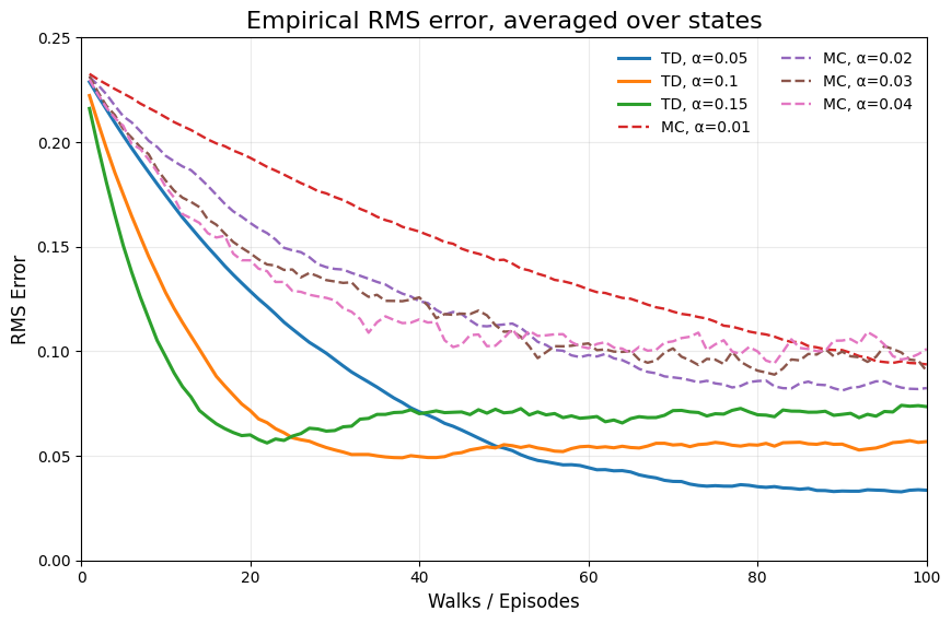
• In practice, TD is faster than MC because it can learn from incomplete episodes.

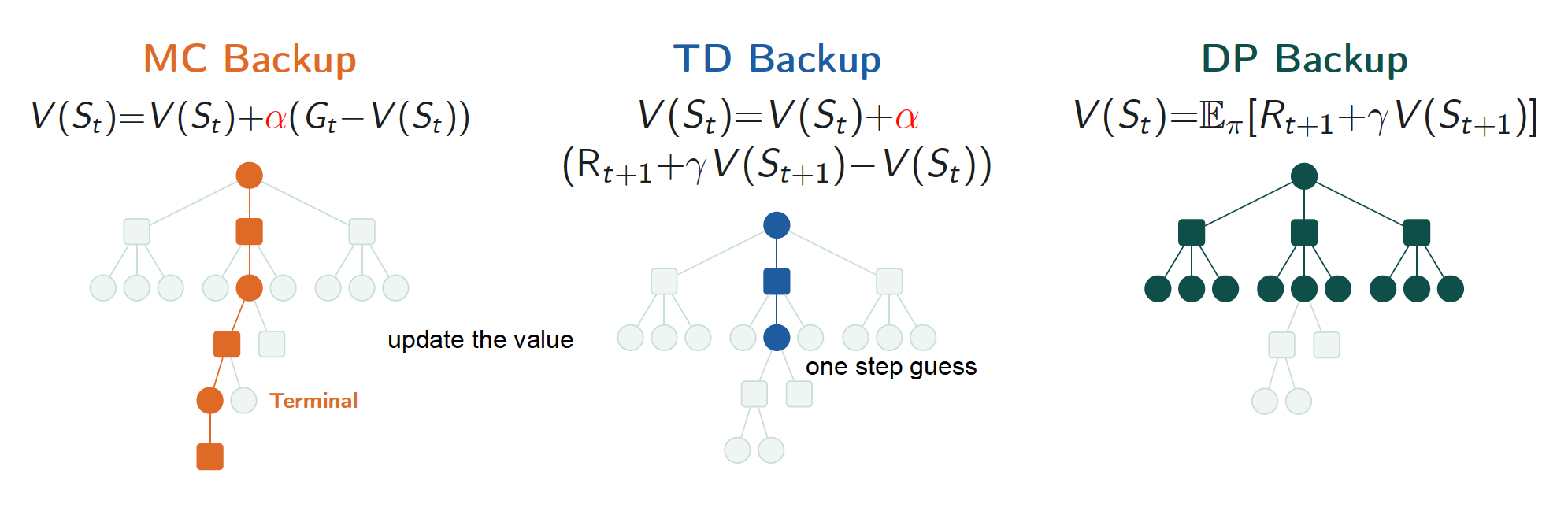
• MC: Full sampled path to the end.
• TD: Just one real step.
• DP: Every branch, weighted by probability, no sampling.

SARSA

$S_t, A_t, R_{t+1}, S_{t+1}, A_{t+1}$

• Follows generalized Policy Iteration.
  • Policy Evaluation: TD Policy Evaluation $Q \approx q_\pi$
  • Policy Improvement: $\epsilon$-greedy policy improvement, allowing exploration.
  • Update happens after every time step.
• Use TD methods for evaluation. $Q(S, A)$
• TD Evaluation + $\epsilon$-greedy Policy Improvement = SARSA

$Q(S_t, A_t) = Q(S_t, A_t) + \alpha [\underbrace{R_{t+1} + \gamma Q(S_{t+1}, A_{t+1})}_{\text{TD target}} - Q(S_t, A_t)]$

• $(S_t, A_t, R_{t+1}, S_{t+1}, A_{t+1})$: transition from one state-action pair to the next.
• The process repeatedly alternates between improving $Q$ and improving the policy.
• The estimates gradually move toward the optimal action-value function $q_*$ and the optimal policy $\pi_*$.
• Unlike classical policy iteration, SARSA does not need to complete policy evaluation before improving the policy.

SARSA Example

• $Q(S_t,A_t)=10$
• $R_{t+1}=2$
• $\gamma=0.9$
• $\alpha=0.5$
• $Q(S_{t+1},A_{t+1})=8$
• TD Target $=2+0.9(8)=9.2$
• TD Error $=9.2-10=-0.8$
• Updated $Q(S_t,A_t)=10+0.5(-0.8)=9.6$

SARSA Algorithm

$$\begin{aligned} &\text{Loop for each episode:} \\ &\quad \text{Initialize} \quad S \\ &\quad \text{Choose} A_t \text{ from } S_t \text{ using policy } \pi \text{ derived from } Q\\ &\quad \text{Loop for each step of the episode:} \\ &\quad \quad \text{Take action} \quad A_{t+1}, \quad \text{observe} \quad R_{t+1}, \quad S_{t+1} \\ &\quad \quad Q(S_t, A_t) \leftarrow Q(S_t, A_t) + \alpha [R_{t+1} + \gamma Q(S_{t+1}, A_{t+1}) - Q(S_t, A_t)] \\ &\quad \quad S_t \leftarrow S_{t+1} \\ &\quad \quad A_t \leftarrow A_{t+1} \\ &\quad \text{Until} \quad S \text{ is terminal} \\ \end{aligned}$$

• As SARSA learns, each episode is completed faster.
• As the Q-values improve, the agent learns better actions for each state and reaches the goal using fewer steps.

Q-Learning

• On-policy: SARSA, behavior policy is the same as the target policy.
• Off-policy: Q-Learning, behavior policy is different from the target policy. $Q(S, A)$
• Update $Q(S_t, A_t)$ toward the value of the alternative, best action.

$Q(S_t, A_t) = Q(S_t, A_t) + \alpha [\underbrace{R_{t+1} + \gamma \max_{a} Q(S_{t+1}, a)}_{\text{TD target}} - Q(S_t, A_t)]$

• The Actual next action is replaced by the Best possible action.

• $Q(S_t, A_t)=10$
• $R_{t+1}=2$
• $\gamma=0.9$
• $\alpha=0.5$
• $Q(S_{t+1}, a_1)=8$
• $Q(S_{t+1}, a_2)=11$
• $Q(S_{t+1}, a_3)=5$
• TD Target $=2+0.9(11)=11.9$
• TD Error $=11.9-10=1.9$
• Updated $Q(S_t, A_t)=10+0.5(1.9)=10.95$

Q-Learning Algorithm

$$\begin{aligned} &\text{Loop for each episode:} \\ &\quad \text{Initialize} \quad S \\ &\quad \text{Loop for each step of the episode:} \\ &\quad \quad A_t \text{ from} S_t \text{ using policy } \pi \text{ derived from } Q\\ &\quad \quad \text{Take action} \quad A_{t+1}, \quad \text{observe} \quad R_{t+1}, \quad S_{t+1} \\ &\quad \quad Q(S_t, A_t) \leftarrow Q(S_t, A_t) + \alpha [R_{t+1} + \gamma \max_{a} Q(S_{t+1}, a) - Q(S_t, A_t)] \\ &\quad \quad S_t \leftarrow S_{t+1} \\ &\quad \text{Until} \quad S \text{ is terminal} \\ \end{aligned}$$

Cliff Walking

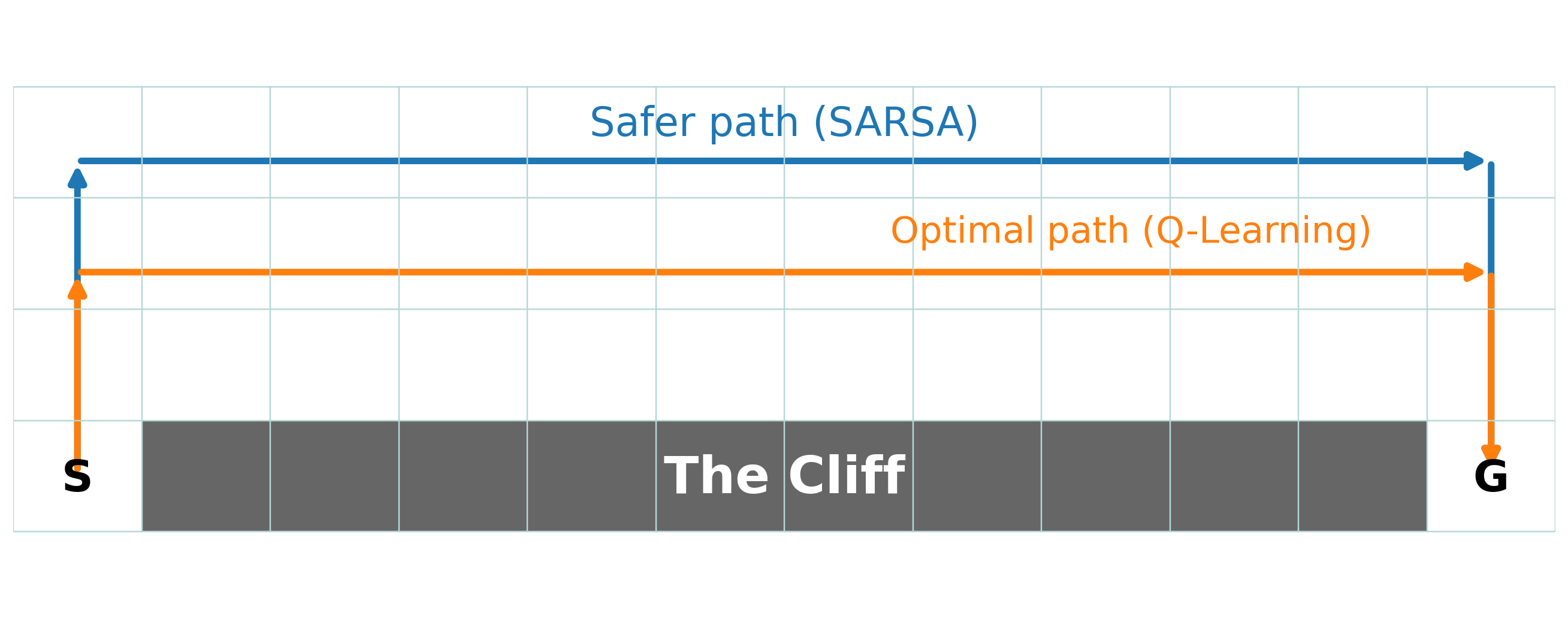
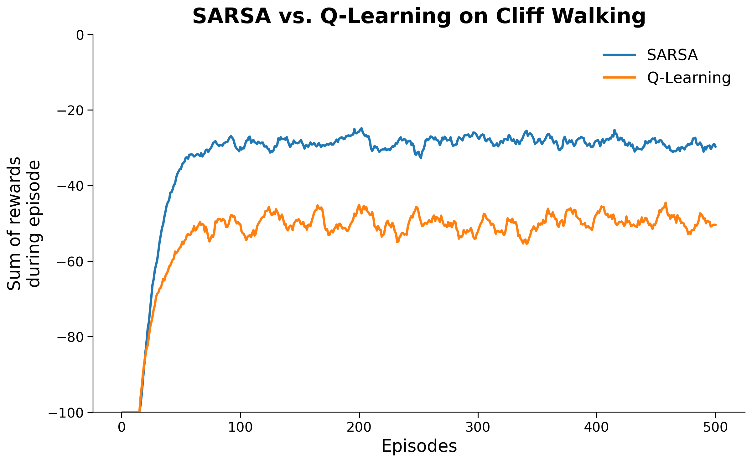
• SARSA (on-policy) accounts for ε-greedy exploration near the cliff and learns the safer route.
• Q-Learning (off-policy) learns the optimal route.
  • but occasionally falls off the cliff during exploration, hurting its online performance

Aspect	SARSA	Q-Learning
Policy type	On-policy	Off-policy
Bootstrap target	$Q(S_{t+1},A_{t+1})$	$\max_a Q(S_{t+1},a)$
Next action used	Action actually taken	Best possible action
Learns	Value of the behavior policy being followed	Optimal policy $\pi_*$
Cliff Walking	Safer path	Optimal but riskier path