본문으로 건너뛰기

"rl" 태그로 연결된 8개 게시물개의 게시물이 있습니다.

모든 태그 보기

RL 008

· 약 9분

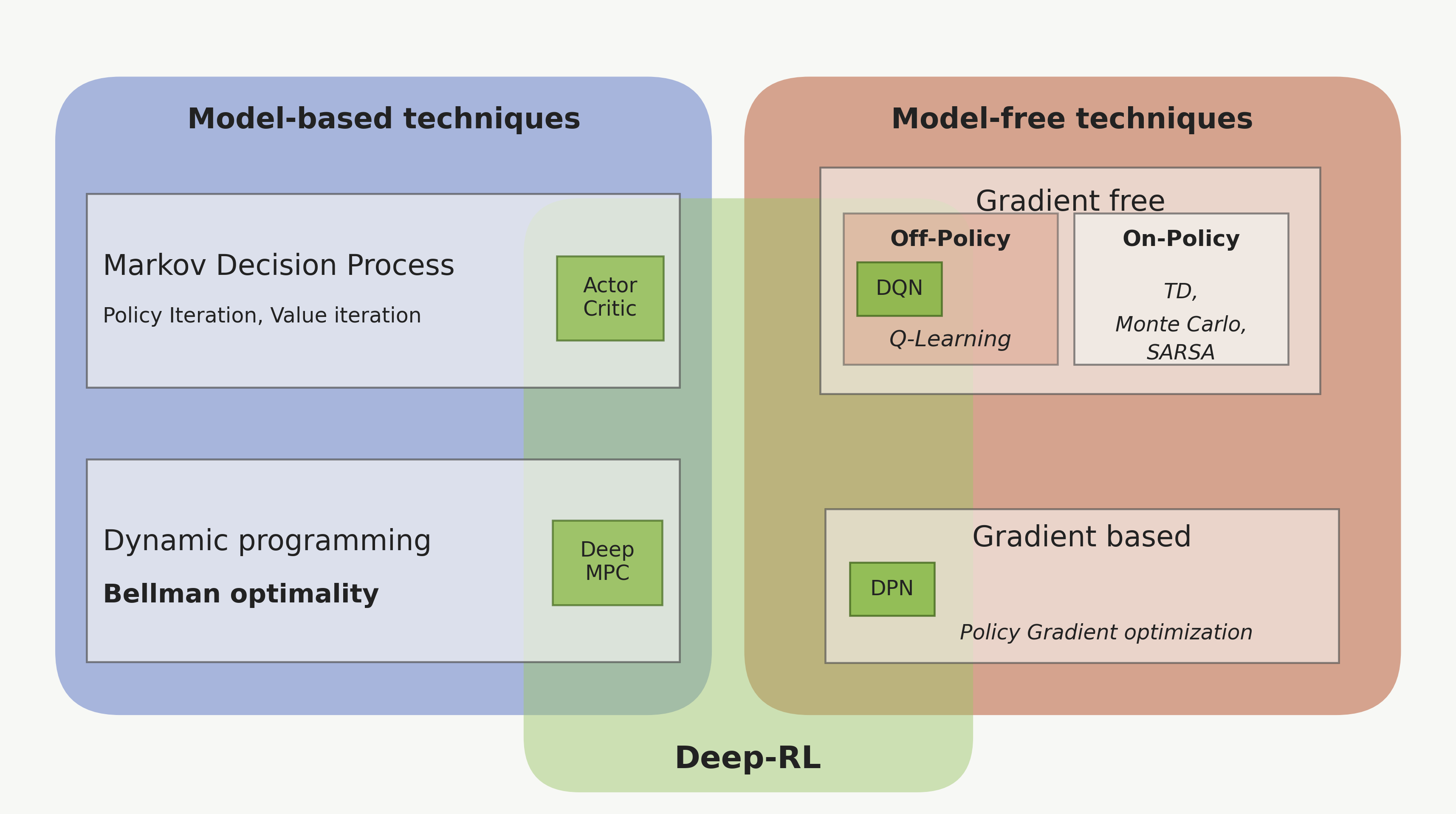
RL Taxonomy​

Drawbacks of previous methods​

  • Large state space:
    • Go: 1017010^{170}
    • Backgammon: 102010^{20}
    • Atari games: 109 to 101110^9 \text{ to } 10^{11}
  • Scale-up model-free based techniques for prediction and control is challenging.
  • Value function used look-up table representation
    • All states has an entry in V(s)V(s)
    • All state-action pair (s,a)(s,a) has an entry in Q(s,a)Q(s,a)
  • Too many state, and stat-action pair to store in memory
  • Slow learning process for each states, due to large space.
  • Each states needs to be explored sufficiently.
  • For large MDPs
    • Function approximation: Almost near optimal value.
    • Estimate value function with function approximation.
      • v^(s,w)≈vπ(s)\hat{v}(s,w) \approx v_\pi(s)
      • q^(s,a,w)≈qπ(s,a)\hat{q}(s,a,w) \approx q_\pi(s,a)
    • Generalize from seen states to unseen states.
    • Using MC or TD learning techniques: Update parameter ww.

Function Approximation​

  • A technique for estimating unknown underlying function using historical or available observations.
  • Assumption: an underlying mapping function exists
    • f(x)≈f^(x)f(x) \approx \hat{f}(x)
  • Function: x→fyx \xrightarrow{f} y

Types of Value Function Approximation​

State-value: state ss → scalar v^(s,w)\hat{v}(s,w)

Action-value (s, a input): state ss and action aa → scalar q^(s,a,w)\hat{q}(s,a,w)

Action-value (s input, all actions out): state ss → q^(s,a1,w),…,q^(s,am,w)\hat{q}(s,a_1,w),\ldots,\hat{q}(s,a_m,w)

  • ww is the parameter vector of the function approximator.
    • e.g. Neural Network weights

Types of Function Approximator​

  • Tabular
    • V-Table: s→v(s)s \rightarrow v(s)
    • Q-Table: (s,a)→q(s,a)(s,a) \rightarrow q(s,a)
  • Decision Trees, Nearest Neighbors
    • s=[speed=49,distance=10]s = [\text{speed} = 49, \text{distance} = 10]
    • s→Decision Tree / KNN→v^(s)s \rightarrow \text{Decision Tree / KNN} \rightarrow \hat{v}(s)
  • Linear Function approximation
    • Linear Combination of Features
    • Values are linear function for features v^(s,w)=wTx(s)\hat{v}(s,w) = w^Tx(s)
    • x(s)=[speeddistancefuel]x(s) = \begin{bmatrix} \text{speed} \\ \text{distance} \\ \text{fuel} \end{bmatrix}
    • v^(s,w)=wTx(s)\hat{v}(s,w) = w^Tx(s)
    • v^(s,w)=w1x1(s)+⋯+wnxn(s)\hat{v}(s,w) = w_1x_1(s) + \cdots + w_n x_n(s)
  • Differentiable function approximation
    • v^(s,w)\hat{v}(s,w) is a differentiable function of ww, can be non-linear in ss
    • e.g. Neural Network, or CNN
      • ∂v^(s,w)∂w\frac{\partial \hat{v}(s,w)}{\partial w}
      • w←w−α∇wLw \leftarrow w - \alpha \nabla_wL
      • Pixels→CNNv^(s)\text{Pixels} \xrightarrow{CNN} \hat{v}(s)

Which FA to use?​

In principle, any FA that fits the RL framework can be used.

FANotes
TabularEasy; not scalable; does not generalise
LinearRequires good features
Differentiable (better choice)Scalable; not always well understood
Neural NetworksPerforms well
Deep Neural NetworksPopular choice; performs well
  • Need training methods that are suitable for non-stationary data.

ANN​

Logistic Regression​

L(a,y)=−ylog⁡(a)−(1−y)log⁡(1−a)\mathcal{L}(a, y) = -y \log(a) - (1-y) \log(1-a)

  • Loss function for Logistic Regression

Gradient Descent​

Goal: Find ww tht minimize J(w)J(w) or find a local minimum of J(w)J(w).

  • An iterative approach for error correction.
  • For one sample, L(a,y)=−ylog⁡(a)−(1−y)log⁡(1−a)\mathcal{L}(a, y) = -y \log(a) - (1-y) \log(1-a)
  • For mm samples,

J(w,b)=1m∑i=1mL(a(i),y(i))J(w, b) = \frac{1}{m} \sum_{i=1}^m \mathcal{L}(a^{(i)}, y^{(i)})

  • Find ww and bb that will minimize J(w,b)J(w, b)
    • min⁡w,bJ(w,b)\min_{w, b} J(w, b)
    • J(w)J(w) is loss function.

w←w−α∂J(w,b)∂w,b←b−α∂J(w,b)∂bw \leftarrow w - \alpha \frac{\partial J(w, b)}{\partial w}, \quad b \leftarrow b - \alpha \frac{\partial J(w, b)}{\partial b}

ΔwJ(w)=(∂J(w)∂w1,…,∂J(w)∂wn)\Delta w J(w) = \big(\frac{\partial J(w)}{\partial w_1}, \ldots, \frac{\partial J(w)}{\partial w_n}\big)

  • Adjust the ww in the direction of the -ve gradient.
    • w=w−αΔw,b=b−αΔbw = w - \alpha \Delta w, \quad b = b - \alpha \Delta b
    • where α\alpha is the learning rate.
    • and, Δw=∂J(w,b)∂w,Δb=∂J(w,b)∂b\Delta w = \frac{\partial J(w, b)}{\partial w}, \quad \Delta b = \frac{\partial J(w, b)}{\partial b}

ANN as a Function Approximator​

  • Need a method to estimate: Δw\Delta w
  • Method to incrementally adjust and update: ww
  • Representation of some aspects of RL environments as feature vector x(s)x(s)
  • Aspects can be approximated: V(s) or Q(s,a)V(s) \text{ or } Q(s, a)
    • Estimate value functions with function approximation.
    • V^(s,w)≈V(s)\hat{V}(s, \color{red}{w}\color{black}) \approx V(s)
    • Q^(s,a,w)≈Q(s,a)\hat{Q}(s, a, \color{red}{w}\color{black}) \approx Q(s, a)
  • A mechanism to plugin MC and TD for function approximation.

Value Function Approximation for policy evaluation​

VFA: Value Function Approximation

  • vπ(s)v_\pi(s) is given, so making it supervised.
  • v^(s,w)\hat{v}(s, w) is estimated value if it follows the policy π\pi by using ANN.
  • x→y^vsyx \rightarrow \hat{y} \quad \text{vs} \quad y (supervised learning)
  • s→v^(s,w)vsvπ(s)s \rightarrow \hat{v}(s, w) \quad \text{vs} \quad v_\pi(s) (Reinforcement learning)

J(w)=Eπ[(vπ(s)−v^(s,w))2] J(w) = \mathbb{E}_\pi[\big(v_\pi(s) - \hat{v}(s, w)\big)^2]

  • Find ww that minimizes J(w)J(w)
    • J(w)J(w): Loss function.
    • v^(s,w)\hat{v}(s, w): Guess from the value function approximation.
    • vπ(s)−v^(s,w)v_\pi(s) - \hat{v}(s, w): Error between the true value and the estimated value.
    • Eπ[⋅]\mathbb{E}_\pi[\cdot]: Expected average over all states ss according to the policy π\pi.
Δw=−12α∇wJ(w)Δw=αEπ[(vπ(s)−v^(s,w))⏟Error∇wv^(s,w)⏟Gradient]\begin{aligned} & \Delta w = -\frac{1}{2} \alpha \nabla_w J(w) \\ & \Delta w = \alpha \mathbb{E}_\pi[\underbrace{\big(v_\pi(s) - \hat{v}(s, w)\big)}_{Error} \underbrace{\nabla_w \hat{v}(s, w)}_{Gradient}] \end{aligned}
  • Δw=\Delta w = Step size X Error X Gradient

VFA with SGD​

Δw=α(vπ(s)−v^(s,w))∇wv^(s,w) \Delta w = \alpha (v_\pi(s) - \hat{v}(s, w)) \nabla_w \hat{v}(s, w)

  • Stochastic Gradient Descent sample the gradient
  • Sample a state randomly, find what vπ(s)v_\pi(s) is, and find the estimate
    • Δw=α[Error at s×Gradient at s]\Delta w = \alpha [\text{Error at } s \times \text{Gradient at } s]
    • Sample sts_t from π\pi, and update ww
  • Expected value update using SGD update is same as full gradient update
    • Random sampling will be eventually the same as full gradient update

Linear Value Function Approximation​

  • Represent Value function (state or action) by a linear combination of features
    • v^(s,w)=x(s)Tw=∑j=0nxj(s)wj\hat{v}(s, w) = x(s)^Tw = \sum_{j=0}^n x_j(s) w_j
  • Loss function: J(w)=Eπ[(vπ(s)−v^(s,w))2]J(w) = \mathbb{E}_\pi[\big(v_\pi(s) - \hat{v}(s, w)\big)^2]

Δw=α(vπ(s)−v^(s,w))⏟Errorx(s)⏟Feature\Delta w = \alpha \underbrace{\big(v_\pi(s) - \hat{v}(s, w)\big)}_{Error} \underbrace{x(s)}_{Feature}

  • Weight update: step size X Error X Feature value
  • SGD converges to global mininum

Incremental methods for prediction​

  • Real-world RL is not supervised, instead, it is guided by rewards.
  • No vπ(s)v_\pi(s) is given.
  • Instead, substitute a target for vπ(s)v_\pi(s)

Δw=α(Gt−v^(st,w))∇wv^(st,w) \Delta w = \alpha(G_t - \hat{v}(s_t, w)) \nabla_w \hat{v}(s_t, w)

  • Monte Carlo updates: target is the return GtG_t

Δw=α(Rt+1+γv^(st+1,w)⏟TD Target−v^(st,w))∇wv^(st,w) \Delta w = \alpha(\underbrace{R_{t+1} + \gamma \hat{v}(s_{t+1}, w)}_{\text{TD Target}} - \hat{v}(s_t, w)) \nabla_w \hat{v}(s_t, w)

  • TD updates: use TD Target

VFA for Monte Carlo​

  • MC return GtG_t is an unbiased, noisy sample of true value vπ(st)v_\pi(s_t)
    • if Gt=3,7,4,6,5,⋯G_t = 3, 7, 4, 6, 5, \cdots
    • but in average, 1N∑i=1NGt(i)≈vπ(s)\frac{1}{N} \sum_{i=1}^N G_t^{(i)} \approx v_\pi(s)
  • ⟨S1,G1⟩,⟨S2,G2⟩,⋯ ,⟨SN,GN⟩\langle S_1, G_1 \rangle, \langle S_2, G_2 \rangle, \cdots, \langle S_N, G_N \rangle is an estimate of vπ(s)v_\pi(s)
    • x→yx \rightarrow y (supervised learning)
    • st→Gts_t \rightarrow G_t (Reinforcement learning)
  • so it learns to v^(s,w)≈Gt\hat{v}(s, w) \approx G_t
Δw=α(Gt−v^(s,w))∇wv^(s,w)Δw=α(Gt−v^(s,w))x(s)\begin{aligned} & \Delta w = \alpha(G_t - \hat{v}(s, w)) \nabla_w \hat{v}(s, w) \\ & \Delta w = \alpha \big(G_t - \hat{v}(s, w)\big) x(s) \end{aligned}
  • In Linear VFA, v^(s,w)=wTx(s)\hat{v}(s,w) = w^Tx(s)
    • x(s)x(s) is the feature vector of state ss
    • ww is the weight vector
    • so ∇wv^(s,w)=∇w(wTx(s))=x(s)\nabla_w \hat{v}(s, w) = \nabla_w (w^Tx(s)) = x(s)
  • Update = Learning rate X Error X state features
Initialize w=0,k=1Loop:Sample k-th episode (sk1,ak1,rk1,...,SkLk) using policy πFor t=1,...Lk:if First Visit to (s) in episode k,thenGt(s)=∑j=tLkγk,jWeight update: w←w−α(Gt−v^(s,w))x(s)k=k+1\begin{aligned} & \text{Initialize } w = 0, k = 1 \\ & Loop: \\ & \quad \text{Sample k-th episode } (s_{k1}, a_{k1}, r_{k1}, ..., S_{kL_k}) \text{ using policy } \pi \\ & \quad \text{For } t = 1, ... L_k: \\ & \quad \quad \text{if First Visit to } (s) \text{ in episode } k, then \\ & \quad \quad \quad G_t(s) = \sum_{j=t}^{L_k} \gamma_{k,j} \\ & \quad \quad \quad \text{Weight update: } \quad w \leftarrow w - \alpha(G_t - \hat{v}(s,w))x(s) \\ & \quad \quad k = k + 1 \\ & \end{aligned}
  • Gt=Rt+1+γRt+2+γ2Rt+3+⋯+γLk−tRLkG_t = R_{t+1} + \gamma R_{t+2} + \gamma^2 R_{t+3} + \cdots + \gamma^{L_k-t} R_{L_k}

VFA for TD Learning​

  • Use bootstrapping and sampling to approximate the target vπv_\pi
    • Sampling: Use a sampled transition St,At,Rt+1,St+1S_t, A_t, R_{t+1}, S_{t+1} instead of computing the full expectation over possible transitions.
    • Bootstrapping: Construct the TD target using the current estimate v^(St+1,w)\hat{v}(S_{t+1}, w), instead of waiting for the complete episodic return.

Rt+1+γv^(St+1,w)R_{t+1} + \gamma \hat{v}(S_{t+1}, w)

  • TD Target is a biased sample of true value vπ(St)v_\pi(S_t)
  • Can use supervised learning on a training set of ⟨S,R⟩\langle S, R \rangle paris
    • ⟨S1,R2+γv^(S2,w)⟩,⟨S2,R3+γv^(S3,w)⟩,⋯ ,⟨ST−1,RT⟩\langle S_1, R_2 + \gamma \hat{v}(S_2, w) \rangle, \langle S_2, R_3 + \gamma \hat{v}(S_3, w) \rangle, \cdots, \langle S_{T-1}, R_T \rangle

Δw=α(R+γv^(s′,w)−v^(s,w))∇wv^(s,w) \Delta w = \alpha(R + \gamma \hat{v}(s', w) - \hat{v}(s, w)) \nabla_w \hat{v}(s, w)

  • Linear VFA + TD(0) for prediction and policy evaluation
  • TD Error: δt=Rt+1+γv^(St+1,w)−v^(St,w)\delta_t = R_{t+1} + \gamma \hat{v}(S_{t+1}, w) - \hat{v}(S_t, w)
  • Δw=αδt∇wv^(St,w)\Delta w = \alpha \delta_t \nabla_w \hat{v}(S_t, w)
    • ∇wv^(s,w)=x(s)\nabla_w \hat{v}(s, w) = x(s)
    • Δw=αδtx(s)\Delta w = \alpha \delta_t x(s)
    • w←w−αδtx(s)w \leftarrow w - \alpha \delta_t x(s)
Initialize w=0Loop:Initialize sSample transition (s,a,r,s′) using policy πWeight update: w←w−α(R+γv^(s′,w)−v^(s,w))x(s)\begin{aligned} & \text{Initialize } w = 0 \\ & Loop: \\ & \quad \text{Initialize } s \\ & \quad \text{Sample transition } (s, a, r, s') \text{ using policy } \pi \\ & \quad \text{Weight update: } \quad w \leftarrow w - \alpha(R + \gamma \hat{v}(s', w) - \hat{v}(s, w))x(s) \\ & \end{aligned}

Overall​

  • Linear VFA: v^(s,w)=wTx(s)\hat{v}(s, w) = w^Tx(s)
  • MC Target = GtG_t
  • TD Target = Rt+1+γv^(s′,w)R_{t+1} + \gamma \hat{v}(s', w)
  • MC: w←w+α(Gt−v^(s,w))x(s)w \leftarrow w + \alpha(G_t - \hat{v}(s, w)) x(s)
  • TD: w←w+α(Rt+1+γv^(s′,w)−v^(s,w))x(s)w \leftarrow w + \alpha(R_{t+1} + \gamma \hat{v}(s', w) - \hat{v}(s, w))x(s)

RL 007

· 약 7분

Temporal-Difference Learning​

Updates a guess towards a guess.

  • Model-free: No MDP Dynamics or Rewards
  • Learns directly from episodes of experience.
  • Bootstrapping: Estimate value function using estimated value from incomplete episodes.
    • Update estimate using another estimate.
  • Updates the estimate of VV immediately after each step.
  • Combines Monte Carlo and Dynamic Programming (Bootstrapping idea).

MC​

V(St)=V(St)+α[Gt⏟Goal−V(St)⏟Previous estimate]V(S_t) = V(S_t) + \alpha [\underbrace{G_t}_{\text{Goal}} - \underbrace{V(S_t)}_{\text{Previous estimate}} ]

  • Update V(St)V(S_t) towards the actual return.
  • α=1n\alpha = \frac{1}{n}: Every-visit MC.
    • gives equal weight to all past samples in the arithmetic mean.
  • Fixed α>1n\alpha > \frac{1}{n}: gives more weight to recent experience and reduces the influence of older episodes faster.
    • α=0.1,V(S)=10\alpha = 0.1, \quad V(S) = 10
    • V(S)←10+0.1(20−10)=11V(S) \leftarrow 10 + 0.1 (20 - 10) = 11
    • V(S)←11+0.1(30−11)=12.9V(S) \leftarrow 11 + 0.1 (30 - 11) = 12.9
    • Move 10% of the way towards the new value.

One-Step Bootstrapping​

TD(0)→TD(λ)→TD(1)≈MC\text{TD}(0) \rightarrow \text{TD}(\lambda) \rightarrow \text{TD}(1) \approx \text{MC}

  • λ\lambda controls how much longer-term return information is used in the TD update.
    • It controls how far into the future TD learns from.
  • λ=0\lambda = 0: uses one-step bootstrapping, corresponding to TD(0).
  • As λ\lambda increases, rewards further into the future have more influence on the update.
  • λ=1\lambda = 1: approaches the Monte Carlo return in episodic tasks.

V(St)=V(St)+α[Rt+1+γV(St+1)⏟TD target−V(St)⏟TD Error]V(S_t) = V(S_t) + \alpha [\underbrace{\underbrace{R_{t+1} + \gamma V(S_{t+1})}_{\text{TD target}} - V(S_t)}_{\text{TD Error}} ]

  • Only one immediate reward is used Rt+1R_{t+1}.
  • Everything after that is replaced by the current guess V(St+1)V(S_{t+1}) instead of actual future rewards.
  • It uses actual reward for the first step and the estimated value/guess for the rest.
MC
Sₜ ──Rₜ₊₁──> Sₜ₊₁ ──Rₜ₊₂──> ... ──> Terminal
│ │
└────────── episode 끝까지 기다림 ────────┘
↓
actual Gₜ
↓
V(Sₜ) update


TD(0)
Sₜ ──Rₜ₊₁──> Sₜ₊₁ ── ? ──> ...
│ │
│ └─ current V(Sₜ₊₁)
│
└── Rₜ₊₁ + γV(Sₜ₊₁)로 즉시 V(Sₜ) update

TD(0) Algorithm​

Loop for each episode:InitializeSLoop for each step of the episode:A←action given by policyπTake actionA,observeR,S′V(S)←V(S)+α[R+γV(S′)−V(S)]S←S′UntilS is terminal\begin{aligned} &\text{Loop for each episode:} \\ &\quad \text{Initialize} \quad S \\ &\quad \text{Loop for each step of the episode:} \\ &\quad \quad A \leftarrow \text{action given by policy} \quad \pi \\ &\quad \quad \text{Take action} \quad A, \quad \text{observe} \quad R, \quad S' \\ &\quad \quad V(S) \leftarrow V(S) + \alpha [R + \gamma V(S') - V(S)] \\ &\quad \quad S \leftarrow S' \\ &\quad \text{Until} \quad S \text{ is terminal} \\ \end{aligned}
  • No need to wait until the end of the episode to update the value function.

MC vs. TD​

AspectMonte Carlo (MC)Temporal-Difference (TD)
Learning sequenceLearns from complete episodesLearns from incomplete episodes
TargetActual return GtG_tEstimated return using bootstrapping
Update timingAfter the episode endsBefore the episode ends / step by step
Future informationUses actual future rewardsUses observed reward(s) + estimated future value
BootstrappingNoYes
BiasUnbiasedBiased
VarianceHighLow
EnvironmentEpisodic / terminating environmentsAlso works in continuing / non-terminating environments
Practical speedSlower updatesFaster updates in practice

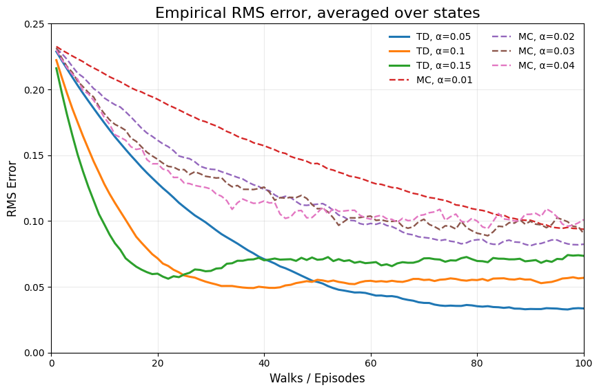
RMS Error Comparison between MC and TD

  • In practice, TD is faster than MC because it can learn from incomplete episodes.

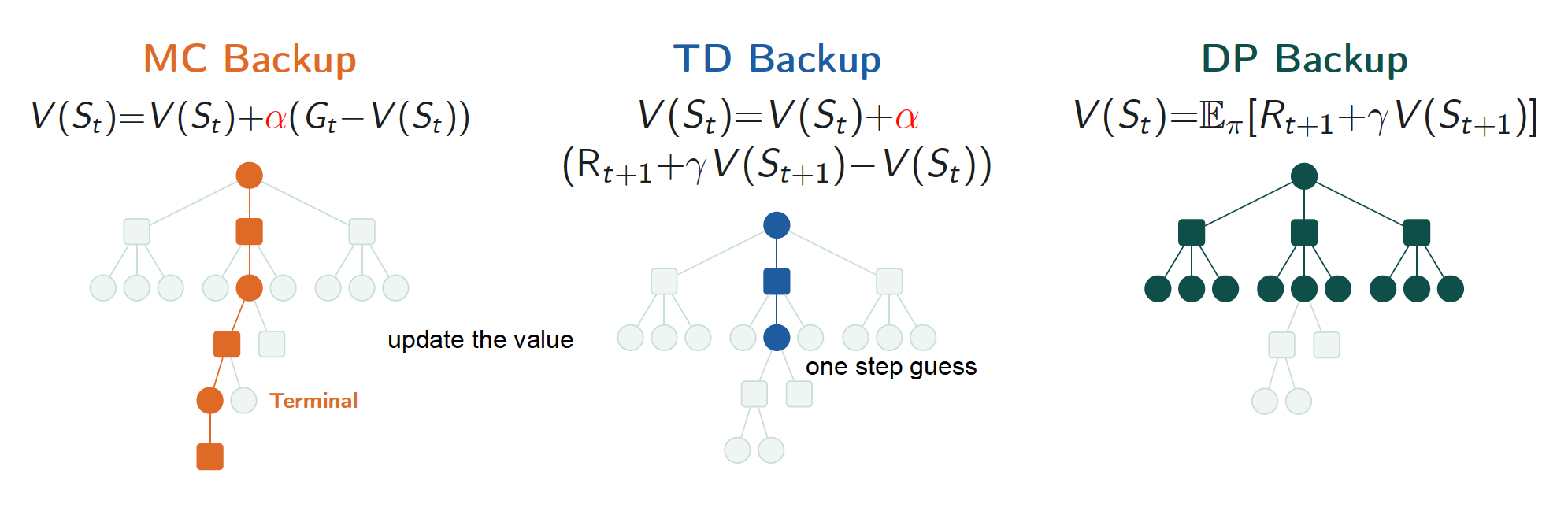
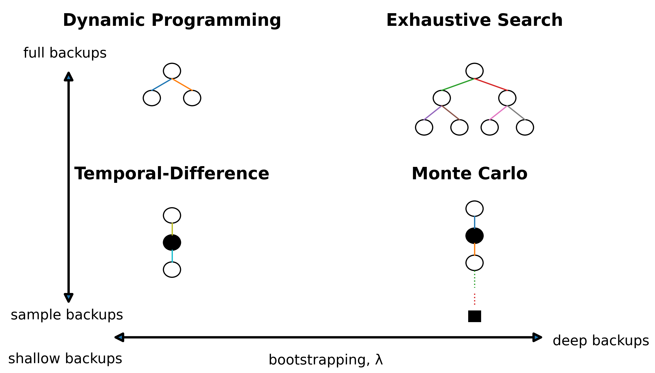
MC, TD, and DP

  • MC: Full sampled path to the end.
  • TD: Just one real step.
  • DP: Every branch, weighted by probability, no sampling.

Backup Methods

SARSA​

St,At,Rt+1,St+1,At+1S_t, A_t, R_{t+1}, S_{t+1}, A_{t+1}

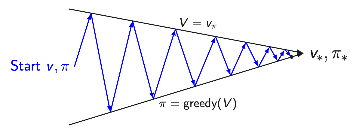
  • Follows generalized Policy Iteration.
    • Policy Evaluation: TD Policy Evaluation Q≈qπQ \approx q_\pi
    • Policy Improvement: ϵ\epsilon-greedy policy improvement, allowing exploration.
    • Update happens after every time step.
  • Use TD methods for evaluation. Q(S,A)Q(S, A)
  • TD Evaluation + ϵ\epsilon-greedy Policy Improvement = SARSA

Q(St,At)=Q(St,At)+α[Rt+1+γQ(St+1,At+1)⏟TD target−Q(St,At)]Q(S_t, A_t) = Q(S_t, A_t) + \alpha [\underbrace{R_{t+1} + \gamma Q(S_{t+1}, A_{t+1})}_{\text{TD target}} - Q(S_t, A_t)]

  • (St,At,Rt+1,St+1,At+1)(S_t, A_t, R_{t+1}, S_{t+1}, A_{t+1}): transition from one state-action pair to the next.
  • The process repeatedly alternates between improving QQ and improving the policy.
  • The estimates gradually move toward the optimal action-value function q∗q_* and the optimal policy π∗\pi_*.
  • Unlike classical policy iteration, SARSA does not need to complete policy evaluation before improving the policy.

SARSA Example​

  • Q(St,At)=10Q(S_t,A_t)=10
  • Rt+1=2R_{t+1}=2
  • γ=0.9\gamma=0.9
  • α=0.5\alpha=0.5
  • Q(St+1,At+1)=8Q(S_{t+1},A_{t+1})=8
  • TD Target =2+0.9(8)=9.2=2+0.9(8)=9.2
  • TD Error =9.2−10=−0.8=9.2-10=-0.8
  • Updated Q(St,At)=10+0.5(−0.8)=9.6Q(S_t,A_t)=10+0.5(-0.8)=9.6

SARSA Algorithm​

Loop for each episode:InitializeSChooseAt from St using policy π derived from QLoop for each step of the episode:Take actionAt+1,observeRt+1,St+1Q(St,At)←Q(St,At)+α[Rt+1+γQ(St+1,At+1)−Q(St,At)]St←St+1At←At+1UntilS is terminal\begin{aligned} &\text{Loop for each episode:} \\ &\quad \text{Initialize} \quad S \\ &\quad \text{Choose} A_t \text{ from } S_t \text{ using policy } \pi \text{ derived from } Q\\ &\quad \text{Loop for each step of the episode:} \\ &\quad \quad \text{Take action} \quad A_{t+1}, \quad \text{observe} \quad R_{t+1}, \quad S_{t+1} \\ &\quad \quad Q(S_t, A_t) \leftarrow Q(S_t, A_t) + \alpha [R_{t+1} + \gamma Q(S_{t+1}, A_{t+1}) - Q(S_t, A_t)] \\ &\quad \quad S_t \leftarrow S_{t+1} \\ &\quad \quad A_t \leftarrow A_{t+1} \\ &\quad \text{Until} \quad S \text{ is terminal} \\ \end{aligned}
  • As SARSA learns, each episode is completed faster.
  • As the Q-values improve, the agent learns better actions for each state and reaches the goal using fewer steps.

Q-Learning​

  • On-policy: SARSA, behavior policy is the same as the target policy.
  • Off-policy: Q-Learning, behavior policy is different from the target policy. Q(S,A)Q(S, A)
  • Update Q(St,At)Q(S_t, A_t) toward the value of the alternative, best action.

Q(St,At)=Q(St,At)+α[Rt+1+γmax⁡aQ(St+1,a)⏟TD target−Q(St,At)] Q(S_t, A_t) = Q(S_t, A_t) + \alpha [\underbrace{R_{t+1} + \gamma \max_{a} Q(S_{t+1}, a)}_{\text{TD target}} - Q(S_t, A_t)]

  • The Actual next action is replaced by the Best possible action.
  • Q(St,At)=10Q(S_t, A_t)=10
  • Rt+1=2R_{t+1}=2
  • γ=0.9\gamma=0.9
  • α=0.5\alpha=0.5
  • Q(St+1,a1)=8Q(S_{t+1}, a_1)=8
  • Q(St+1,a2)=11Q(S_{t+1}, a_2)=11
  • Q(St+1,a3)=5Q(S_{t+1}, a_3)=5
  • TD Target =2+0.9(11)=11.9=2+0.9(11)=11.9
  • TD Error =11.9−10=1.9=11.9-10=1.9
  • Updated Q(St,At)=10+0.5(1.9)=10.95Q(S_t, A_t)=10+0.5(1.9)=10.95

Q-Learning Algorithm​

Loop for each episode:InitializeSLoop for each step of the episode:At fromSt using policy π derived from QTake actionAt+1,observeRt+1,St+1Q(St,At)←Q(St,At)+α[Rt+1+γmax⁡aQ(St+1,a)−Q(St,At)]St←St+1UntilS is terminal\begin{aligned} &\text{Loop for each episode:} \\ &\quad \text{Initialize} \quad S \\ &\quad \text{Loop for each step of the episode:} \\ &\quad \quad A_t \text{ from} S_t \text{ using policy } \pi \text{ derived from } Q\\ &\quad \quad \text{Take action} \quad A_{t+1}, \quad \text{observe} \quad R_{t+1}, \quad S_{t+1} \\ &\quad \quad Q(S_t, A_t) \leftarrow Q(S_t, A_t) + \alpha [R_{t+1} + \gamma \max_{a} Q(S_{t+1}, a) - Q(S_t, A_t)] \\ &\quad \quad S_t \leftarrow S_{t+1} \\ &\quad \text{Until} \quad S \text{ is terminal} \\ \end{aligned}

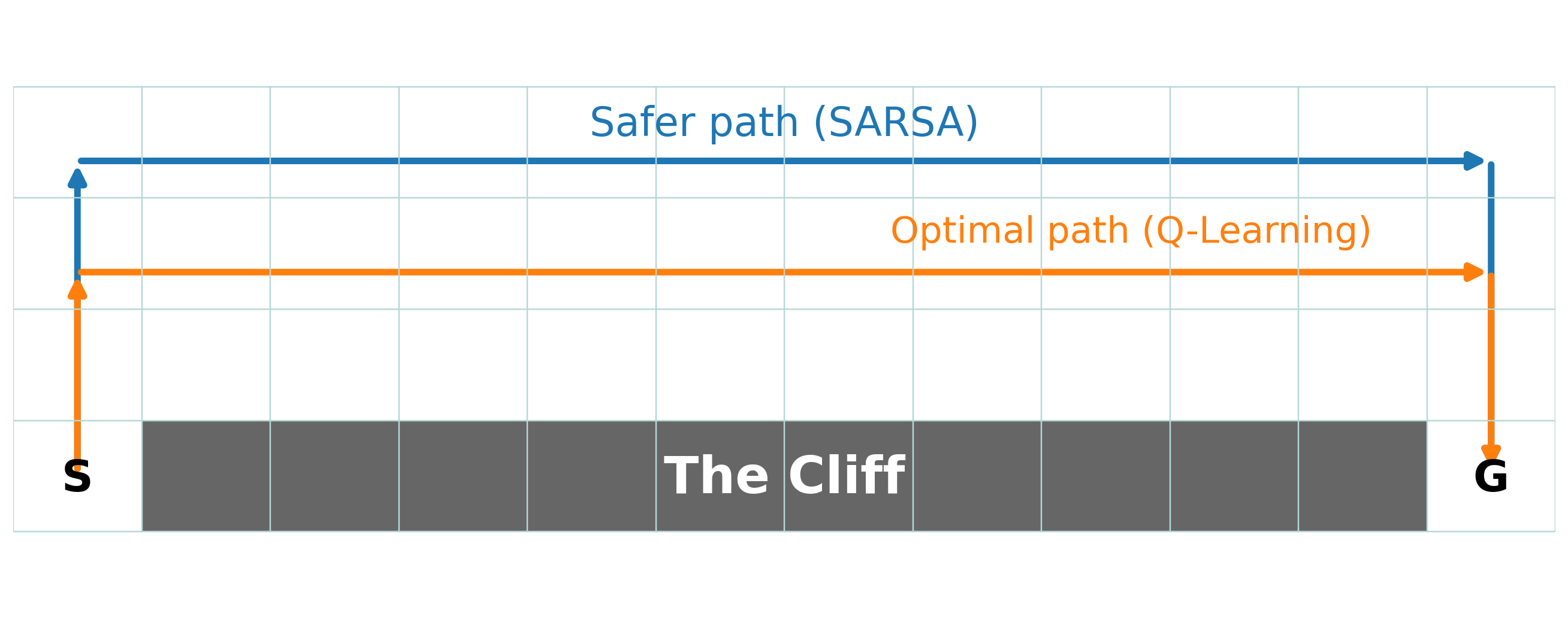
Cliff Walking​

Cliff Walking

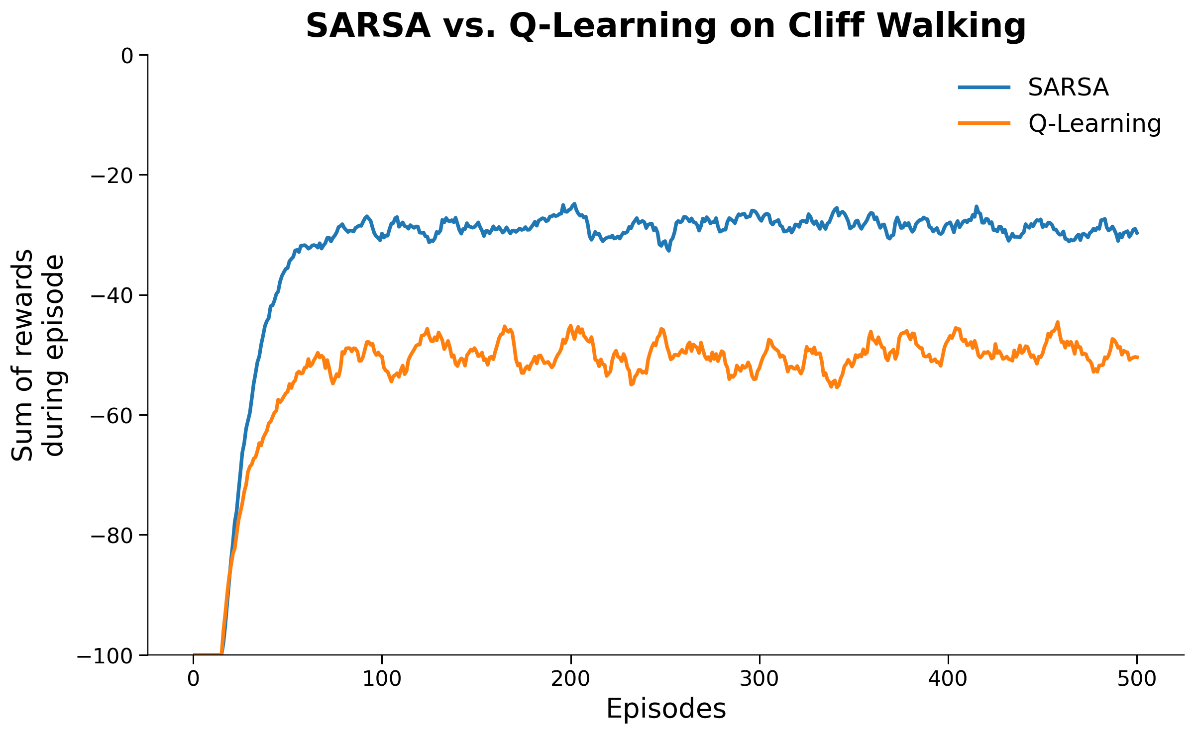
  • SARSA (on-policy) accounts for ε-greedy exploration near the cliff and learns the safer route.
  • Q-Learning (off-policy) learns the optimal route.
    • but occasionally falls off the cliff during exploration, hurting its online performance

Cliff Walking Rewards

AspectSARSAQ-Learning
Policy typeOn-policyOff-policy
Bootstrap targetQ(St+1,At+1)Q(S_{t+1},A_{t+1})max⁡aQ(St+1,a)\max_a Q(S_{t+1},a)
Next action usedAction actually takenBest possible action
LearnsValue of the behavior policy being followedOptimal policy π∗\pi_*
Cliff WalkingSafer pathOptimal but riskier path

RL 006

· 약 12분

Known MDP vs Unknown MDP​

AspectKnown MDPUnknown MDP
Environment Knowledge (P,RP, R)Full knowledge of state transition dynamics PP and reward function RRPP and RR are unknown; agent must explore the environment
Problem ApproachWell-defined optimization problem →\rightarrow Pure planning via computationTrial-and-error interaction →\rightarrow Must learn and optimize simultaneously
Primary GoalDirectly compute the optimal policy (π∗\pi_*)Learn and optimize policies without prior model knowledge
Representative MethodsValue Iteration, Policy Iteration (Dynamic Programming)Monte Carlo, Q-Learning, SARSA (Reinforcement Learning)
ParadigmModel-based (Planning)Model-free (Reinforcement Learning)

Model-based vs Model-free​

AspectModel-Based LearningModel-Free Learning
Model Access (P,RP, R)Has full access to transition dynamics PP and reward function RRNo access to environment dynamics (PP and RR are unknown)
Optimization ApproachDirect mathematical computation and planning using the known modelDirect learning and trial-and-error optimization through interaction
Estimation SourceComputes values and optimal policy π∗\pi_* via dynamic programming equationsEstimates vπ,qπv_\pi, q_\pi, and π∗\pi_* directly from sampled experience
Computation vs. SamplingPure computation / Planning (requires no real-time environment sampling)Sample-based learning (requires trajectories / episodic experience)
Typical MethodsPolicy Iteration, Value Iteration (DP)Monte Carlo Methods, TD Learning, Q-Learning, SARSA

Monte Carlo Methods​

  • A Computational technique that uses random sampling and statistical methods to solve complex problems and estimate numerical results.
    • Named after the Monte Carlo Casino in Monaco.
    • It means Estimate an unknown quantity by sampling, and averaging what you observe.
  • Used fo any estimation method whose operation involves a significant random component.
  • Used in mathematics, physics, engineering, finance, computer science, etc.
  • It is particularly valuable when an analytical solution is difficult or impossible to obtain.

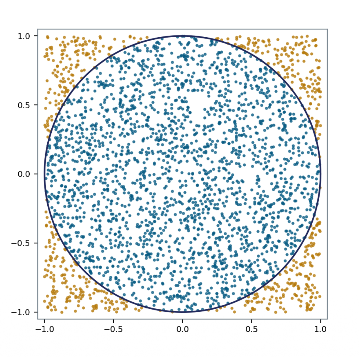
Estimating π\pi by Sampling (Monte Carlo Simulation)​

  • Mechanism:
    • Generate uniform random points (x,y)∈[−1,1]×[−1,1](x, y) \in [-1, 1] \times [-1, 1].
    • Count points falling inside the unit circle (x2+y2≤1x^2 + y^2 \le 1).
    • Estimate π\pi via area proportions:
AreacircleAreasquare=π4π≈4×#points inside circle#total points\begin{aligned} \frac{\text{Area}_{circle}}{\text{Area}_{square}} = \frac{\pi}{4} \\ & \pi \approx 4 \times \frac{\text{\#points inside circle}}{\text{\#total points}} \end{aligned}
  • Empirical Validation:
    • Total samples (nn): 30003000 points
    • Estimated value: π=3.1386666666666665\pi = 3.1386666666666665
    • Relative error: −0.0931%-0.0931\% from true value (≈3.14159265\approx 3.14159265)

Monte Carlo

Monte Carlo Prediction​

vπ(s)=Eπ[Gt∣St=s]≈1N∑i=1N(s)G(i)v_\pi(s) = \mathbb{E}_{\pi}[G_t | S_t = s] \approx \frac{1}{N} \sum_{i=1}^{N(s)} G^{(i)}

  • 1N∑i=1N(s)G(i)\frac{1}{N} \sum_{i=1}^{N(s)} G^{(i)}: Mean of the returns/rewards
  • Model-Free Learning: Operates without prior knowledge of transition dynamics PP or reward function RR.
  • Learning from Complete Episodes: Learns state-value functions vπv_\pi exclusively from full trajectories under policy π\pi. Only works for episodic tasks where termination at step TT is guaranteed.
  • No Bootstrapping: Does not update estimates using other value estimates v(s′)v(s'); instead, updates rely solely on actual empirical returns observed at the end of the episode.
  • Empirical Mean Returns: The value of state ss is estimated by the sample average of all observed returns starting from ss:

An Episode of Experience & Return Formulation​

  • Trajectory Structure: S0→A0,R1S1→A1,R2S2⋯→AT−1,RTSTS_0 \xrightarrow{A_0, R_1} S_1 \xrightarrow{A_1, R_2} S_2 \dots \xrightarrow{A_{T-1}, R_T} S_T
  • Discounted Return (GtG_t): Gt=Rt+1+γRt+2+γ2Rt+3+⋯+γT−t−1RTG_t = R_{t+1} + \gamma R_{t+2} + \gamma^2 R_{t+3} + \dots + \gamma^{T-t-1} R_T
  • Discount Factor (γ=1\gamma = 1): For episodic tasks with terminal-only rewards (such as Blackjack), setting γ=1\gamma = 1 is standard practice because the episode length is finite.

First-Visit Monte Carlo​

  • First-Visit MC estimates the value function V(s)V(s) by averaging returns following only the first occurrence of state ss within each sampled episode.
  • Algorithmic Flow:
    • Initialize counters N(s)←0N(s) \leftarrow 0 and accumulate returns: G(s)←0∀s∈SG(s) \leftarrow 0 \quad \forall s \in S
    • Sample a complete episode i={Si,0,Ai,1,Ri,2,…,Si,Ti}i = \{S_{i,0}, A_{i,1}, R_{i,2}, \dots, S_{i,T_i}\} generated under policy π\pi
    • Compute return Gi,t=∑k=t+1Tiγk−t−1Ri,kG_{i,t} = \sum_{k=t+1}^{T_i} \gamma^{k-t-1} R_{i,k} from step tt to termination.
    • Only for the first time step tt where state ss appears in episode ii:
      • N(s)←N(s)+1N(s) \leftarrow N(s) + 1 (Increment counter for total first visits)
      • G(s)←G(s)+Gi,tG(s) \leftarrow G(s) + G_{i,t} (Increment total return)
      • V(s)←G(s)N(s)V(s) \leftarrow \frac{G(s)}{N(s)} (Update the value by mean return)

A→R1=1B→R2=2A→R3=1C→R4=1terminalA \xrightarrow{R_1=1} B \xrightarrow{R_2=2} A \xrightarrow{R_3 = 1} C \xrightarrow{R_4 = 1} \text{terminal}

State sN(s)N(s)G(s)G(s)V(s)=G(s)N(s)V(s) = \frac{G(s)}{N(s)}
A199.00
B188.00
C155.00

Every-Visit Monte Carlo​

  • Every-Visit MC treats every single occurrence of state ss within an episode as a valid data sample, accumulating its corresponding return into the empirical mean.
  • Algorithmic Flow:
    • Initialize counters N(s)←0N(s) \leftarrow 0 and accumulate returns: G(s)←0∀s∈SG(s) \leftarrow 0 \quad \forall s \in S
    • Sample a complete episode i={Si,0,Ai,1,Ri,2,…,Si,Ti}i = \{S_{i,0}, A_{i,1}, R_{i,2}, \dots, S_{i,T_i}\} generated under policy π\pi
    • Compute return Gi,t=∑k=t+1Tiγk−t−1Ri,kG_{i,t} = \sum_{k=t+1}^{T_i} \gamma^{k-t-1} R_{i,k} from step tt to termination.
    • For each time step tt where state ss appears in episode ii:
      • N(s)←N(s)+1N(s) \leftarrow N(s) + 1 (Increment counter for total visits)
      • G(s)←G(s)+Gi,tG(s) \leftarrow G(s) + G_{i,t} (Increment total return)
      • V(s)←G(s)N(s)V(s) \leftarrow \frac{G(s)}{N(s)} (Update the value by mean return)

A→R1=1B→R2=2A→R3=1C→R4=1terminalA \xrightarrow{R_1=1} B \xrightarrow{R_2=2} A \xrightarrow{R_3 = 1} C \xrightarrow{R_4 = 1} \text{terminal}

State sN(s)N(s)G(s)G(s)V(s)=G(s)N(s)V(s) = \frac{G(s)}{N(s)}
A29+6=157.50
B188.00
C155.00
DimensionFirst-Visit MCEvery-Visit MC
Returns used per episodeOnly the first occurrenceEvery occurrence
Sample independenceIndependent across episodes (i.i.d.)Correlated within an episode (mitigated by sampling)
Bias (finite samples)UnbiasedBiased, but bias→0\text{bias} \to 0
ConvergenceConsistent (Law of Large Numbers)Consistent (as episodes→∞\text{episodes} \to \infty)
ImplementationRequires a "seen this episode?" checkSimpler — no check needed
Practical UseStandard theoretical baselineFrequently preferred (uses all available data)

Incremental Mean​

μk=1k∑j=1kxj\mu_k = \frac{1}{k} \sum_{j=1}^{k} x_j

μk+1=1k+1∑j=1k+1xj=1k+1(∑j=1kxj+xk+1)=1k+1(kμk+xk+1)=μk+1k+1(xk+1−μk)\begin{aligned} \mu_{k+1} &= \frac{1}{k+1} \sum_{j=1}^{k+1} x_j \\ &= \frac{1}{k+1} \left( \sum_{j=1}^{k} x_j + x_{k+1} \right) \\ &= \frac{1}{k+1} \left( k \mu_k + x_{k+1} \right) \\ &= \mu_k + \frac{1}{k+1} (x_{k+1} - \mu_k) \end{aligned}
  • New estimate = Old estimate + step-size * (new sample - old estimate).
  • Memory efficient: Only need to store the old estimate (μk\mu_k) and the number of visits (kk).

Incremental Monte Carlo​

  • Updates the value function V(s)V(s) incrementally after each trajectory without requiring memory to store individual past returns.
  • Algorithmic Flow:
    • Initialize N(s)←0N(s) \leftarrow 0 and V(s)←0V(s) \leftarrow 0 for all s∈Ss \in S.
    • Episode sampling: Execute episode ii under policy π\pi and compute returns Gi,t=∑k=t+1Tiγk−t−1RkG_{i,t} = \sum_{k=t+1}^{T_i} \gamma^{k-t-1} R_{k}.
    • Incremental update: For each visited state ss at time step tt:
      • N(s)←N(s)+1N(s) \leftarrow N(s) + 1 (Increment counter for total visits)
      • V(s)←V(s)+α(Gi,t−V(s))V(s) \leftarrow V(s) + \alpha (G_{i,t} - V(s)) (Update the value by mean return)
      • Where Gi,t−V(s)G_{i,t} - V(s) represents the temporal difference (TD) error between the sampled return target and the current estimate.
  • Choice step size α\alpha
    • α=1N(s)\alpha = \frac{1}{N(s)}: Replicates the exact empirical sample-average of Every-Visit MC where all observed samples receive equal weight.
    • α=constant\alpha = \text{constant}: Implements an exponential recency-weighted running average that decays outdated experience, making it suited for non-stationary environments where MDP dynamics change over time.
  • Cons:
    • Requires a significant number of episodes to converge to the true value function.
    • Requires to terminate the episode.

Model-free Control​

  • The MDP model is unknown, or too large/complex to use directly.
  • But experience can be sampled.
  • Applications:
    • Robo soccer
    • Autonomous vehicles
    • Robotics
    • Game playing
    • Recommender systems
    • Finance & portfolio management

On-Policy vs Off-Policy​

DimensionOn-Policy LearningOff-Policy Learning
DefinitionEvaluates and improves the exact same policy currently used to generate action decisionsEvaluates/improves a target policy (π\pi) while behaving via a different behavior policy (bb)
Data GenerationTrajectories must be generated by the current active policy π\piTrajectories can come from exploratory policies, historical logs, or human demonstrations
Exploration Trade-offMust balance exploration directly within the target policy (e.g., ϵ\epsilon-greedy)Separates exploration (behavior policy) from exploitation/optimality (target policy)
Representative AlgorithmsGLIE Monte Carlo Control, SARSAQ-Learning, Deep Q-Networks (DQN)

General Policy Iteration​

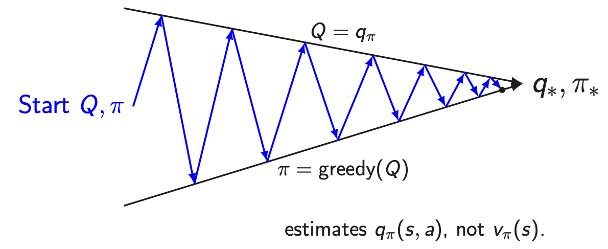
  • Alternates between Policy Evaluation (V≈vπV \approx v_\pi or Q≈qπQ \approx q_\pi) and Policy Improvement (π←greedy\pi \leftarrow \text{greedy}).
  • This interplay drives the system asymptotically toward the optimal pair (v∗,π∗)(v_*, \pi_*) or (q∗,π∗)(q_*, \pi_*).

π′(s)=argmaxa∈A(R(s,a)+γ∑s′∈SP(s′∣s,a)V(s′))\pi'(s) = \text{argmax}_{a \in A} \big( \mathcal{R}(s, a) + \gamma \sum_{s' \in S} \mathcal{P}(s' | s, a) V(s') \big)

  • Why V(s)V(s) Fails in Model-Free Settings:
    • Finding the maximizing action over V(s)V(s) strictly requires the transition model P(s′∣s,a)P(s' \mid s, a) and reward function R(s,a)R(s, a).
    • In Model-Free RL, these dynamics are unavailable; hence, V(s)V(s) alone cannot guide policy updates without an explicit environment model.

GPI

π′(s)=argmaxa∈AQ(s,a)\pi'(s) = \text{argmax}_{a \in A}Q(s,a)

  • Model-Free Advantage:
    • By estimating Q(s,a)Q(s, a) directly through sample episodes, policy improvement requires no knowledge of PP or RR.
    • This fundamental shift makes Q(s,a)Q(s, a) estimation the standard paradigm for Model-Free Control (Monte Carlo Control, SARSA, Q-Learning).
V(s)V(s)Q(s,a)Q(s, a)
QuestionHow good is this state?How good is this action in this state?
Includes Action?NoYes
Policy EvaluationVery suitableSlightly more difficult
Policy ImprovementRequires a modelDirectly possible
Model-Free ControlInconvenientVery suitable

GPI with Q

  • This is why MC Control estimates qπ(s,a)q_\pi(s,a), not vπ(s)v_\pi(s).

Exploration Problem​

a=arg⁡max⁡aQ(s,a)a = \arg\max_a Q(s,a)
  • A greedy agent always chooses the action with the highest current estimated value.
  • But what if the current Q(s,a)Q(s,a) estimates are inaccurate?

Mystery Box Example​

Initially,

Q(red)=0,Q(blue)=0Q(\text{red}) = 0, \qquad Q(\text{blue}) = 0
  1. Open the red box:
    R=0→Q(red)=0R = 0 \rightarrow Q(\text{red}) = 0

  2. Open the blue box:
    R=+1→Q(blue)=1R = +1 \rightarrow Q(\text{blue}) = 1

  3. Keep opening the blue box:
    R=+1,+3,+2,…→Q(blue)≈2R = +1, +3, +2, \ldots \rightarrow Q(\text{blue}) \approx 2

  4. A purely greedy agent now keeps choosing the blue box because
    Q(blue)>Q(red)Q(\text{blue}) > Q(\text{red}).

  5. However, the red box may actually be better. For example,
    E[R∣red]=5\mathbb{E}[R \mid \text{red}] = 5.

    The agent does not know this because it sampled the red box only once.

Exploitation vs. Exploration​

  • Exploitation: Choose the action that currently has the highest estimated value.
  • Exploration: Try less-sampled or unfamiliar actions to discover whether they may actually be better.
  • In this example, the agent should occasionally explore the red box because it has not been sampled enough to confidently conclude that it is worse.

ϵ\epsilon-Greedy Exploration​

π(a∣s)={greedy action with high probabilityrandom action with probability ϵ\pi(a|s) = \begin{cases} \text{greedy action \quad with high probability} \\ \text{random action \quad with probability $\epsilon$} \\ \end{cases}
  • if ϵ=0.1\epsilon = 0.1, then the agent will choose the greedy action with probability 0.90.9 (Exploitation)
  • And the random action with probability 0.10.1 (Exploration).
  • Policy Improvement Theorem:
    • for any ϵ\epsilon-greedy policy π\pi
    • The ϵ\epsilon-greedy policy π′\pi' is as good or better than the original policy π\pi: vπ′(s)≥vπ(s)v_{\pi'}(s) \geq v_{\pi}(s)

Monte Carlo Control​

  • Traditional Policy Iteration:
    • Fix the policy π\pi.
    • Evaluate the current policy until QQ is sufficiently close to qπ(s,a)q_\pi(s,a).
    • Improve the policy using the estimated action values.
    • Repeat policy evaluation and policy improvement.
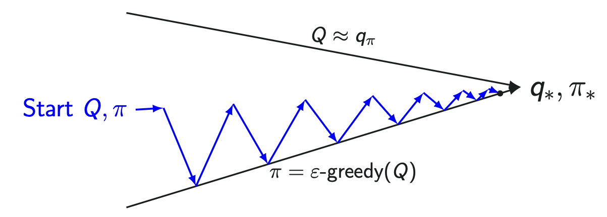
  • Monte Carlo Control:
    • Perform MC Policy Evaluation after every episode.
    • Improve the policy using ϵ\epsilon-greedy after every episode.
    • Q1→π1=ϵ-greedy(Q1)Q_1 \rightarrow \pi_1 = \epsilon\text{-greedy}(Q_1)
    • Q2→π2=ϵ-greedy(Q2)Q_2 \rightarrow \pi_2 = \epsilon\text{-greedy}(Q_2)
    • ⋯\cdots
    • Eventually approaches (q∗,π∗)(q_*, \pi_*) under appropriate convergence conditions.

MC Control

Evaluate a little→Improve→Evaluate a little→Improve→⋯\text{Evaluate a little} \rightarrow \text{Improve} \rightarrow \text{Evaluate a little} \rightarrow \text{Improve} \rightarrow \cdots

GLIE​

Greedy in the Limit with Infinite Exploration

  1. lim⁡k→∞Nk(s,a)=∞\lim_{k \to \infty} N_k(s,a) = \infty
  2. lim⁡k→∞πk(a∣s)=1(a=arg max⁡a′∈AQk(s,a′))\lim_{k \to \infty} \pi_k(a|s) = 1(a = \argmax_{a' \in A} Q_k(s,a'))
  • Explore enough early -> Explore less over time -> Eventually greedy.
    • Nk(s,a)N_k(s,a): How many times the state-action pair (s,a)(s,a) has been visited in the kk-th episode.
    • πk→greedy(Qk)\pi_k \rightarrow \text{greedy}(Q_k)
  • Infinite exploration first, greedy behavior in the limit.

GILE Monte Carlo Control​

  • Algorithm flow:
    • Run episode k={S0,A0,R1,…,ST}k = \{S_0, A_0, R_1, \dots, S_{T}\} with policy πk\pi_k.
    • For each state-action pair (s,a)(s,a) in the episode:
      • Nk(s,a)←Nk(s,a)+1N_k(s,a) \leftarrow N_k(s,a) + 1
      • Qk(s,a)←Qk(s,a)+1Nk(s,a)(Gk−Qk(s,a))Q_k(s,a) \leftarrow Q_k(s,a) + \frac{1}{N_k(s,a)} (G_k - Q_k(s,a))
    • Improve the policy based on the new QQ value.
      • ϵ←1k\epsilon \leftarrow \frac{1}{k}
      • π←ϵ-greedy(Q)\pi \leftarrow \epsilon\text{-greedy}(Q)
    • Repeat until convergence.
  • old estimate + step-size * (new sample - old estimate).
    • old estimate = Q(St,At)Q(S_t, A_t)
    • new sample = GtG_t
    • step-size = 1Nk(s,a)\frac{1}{N_k(s,a)}
  • Run Episode → Update Q → Reduce ϵ\epsilon → Improve Policy

DP vs MC​

  • Dynamic Programming:
    • Model-based
    • Bootstrapping: Updating a value estimate using another estimated value instead of waiting for the final outcome.
    • Lower variance
  • Monte Carlo:
    • Model-free
    • No bootstrapping: It uses rewards that actually occurred, not an estimated value of the next state.
    • Uses complete sampled returns
    • Requires episodic tasks
    • Higher variance

RL 005

· 약 7분

MDP​

(S,A,P,R,γ)(\mathcal{S}, \mathcal{A}, \mathcal{P}, \mathcal{R}, \gamma)

  • At each time step tt, the agent observes state St∈SS_t \in \mathcal{S} and chooses action At∈AA_t \in \mathcal{A}
  • Receives reward Rt+1∈RR_{t+1} \in \mathcal{R}
  • Transitions to a new state St+1S_{t+1}

Transition Dynamics​

Transition Probability

  • How the environment responds to an action, independent of the agent's policy
  • Policy: Whether to brake or accelerate when the traffic light is yellow.
  • Transition Dynamics: How much the car decelerates after braking, and what the resulting next state is.

P(s′∣s,a)=P(St+1=s′∣St=s,At=a)P(s'|s,a) = P(S_{t+1} = s'|S_t = s, A_t = a)

Policy​

  • A policy is the agent’s rule for choosing actions.
  • It tells the agent what action to take in a given state.
  • It defines agent's behavior.

Deterministic Policy:π(s)=a\text{Deterministic Policy}: \pi(s) = a

  • Direct mapping, and no randomness
  • All probability on one action

Stochastic Policy:π(a∣s)=P(At=a∣St=s)\text{Stochastic Policy}: \pi(a|s) = P(A_t = a | S_t = s)

  • A probability distribution over actions.
  • More general, all four Bellman Equations are stochastic, use π(a∣s)\pi(a|s) to represent the policy.
  • Policy is what the agent controls.

Value Functions​

vπ(s)=Eπ[Rt+1+γvπ(St+1)∣St=s]v_\pi(s) = \mathbb{E}_\pi[R_{t+1} + \gamma v_\pi(S_{t+1}) | S_t = s]

  • How good is this state?
  • Eπ[Gt∣St=s]\mathbb{E}_\pi[G_t | S_t = s]

qπ(s,a)=Eπ[Rt+1+γvπ(St+1)∣St=s,At=a]q_\pi(s,a) = \mathbb{E}_\pi[R_{t+1} + \gamma v_\pi(S_{t+1}) | S_t = s, A_t = a]

  • How good is this action in this state?
  • Eπ[Gt∣St=s,At=a]\mathbb{E}_\pi[G_t | S_t = s, A_t = a]

vπ(s)=∑a∈Aπ(a∣s)qπ(s,a)v_\pi(s) = \sum_{a \in \mathcal{A}} \pi(a|s) q_\pi(s,a)

  • The average value of the actions, weighted by the probability of choosing each action.
    • a1a_1 is brake
    • a2a_2 is accelerate
    • vπ(s)=0.8∗10+0.2∗20=10v_\pi(s) = 0.8 * 10 + 0.2 * 20 = 10
qπ(s,a)=R(s,a)+γ∑s′∈SP(s′∣s,a)vπ(s′)q_\pi(s,a) = \mathcal{R}(s,a) + \gamma \sum_{s' \in \mathcal{S}} P(s'|s,a) v_\pi(s')
  • The value of taking action aa in state ss: the immediate reward plus the discounted expected value of the possible next states.

Four Types of Bellman Equations​

vπ(s)=∑aπ(a∣s)qπ(s,a)qπ(s,a)=R(s,a)+γ∑s′P(s′∣s,a)vπ(s′)vπ(s)=∑aπ(a∣s)[R(s,a)+γ∑s′P(s′∣s,a)vπ(s′)]qπ(s,a)=R(s,a)+γ∑s′P(s′∣s,a)∑a′π(a′∣s′)qπ(s′,a′)\begin{aligned} &v_\pi(s) = \sum_{a} \pi(a|s) q_\pi(s,a) \\ &q_\pi(s,a) = \mathcal{R}(s,a) + \gamma \sum_{s'} P(s'|s,a) v_\pi(s') \\ &v_\pi(s) = \sum_{a} \pi(a|s) \left[ \mathcal{R}(s,a) + \gamma \sum_{s'} P(s'|s,a) v_\pi(s') \right] \\ &q_\pi(s,a) = \mathcal{R}(s,a) + \gamma \sum_{s'} P(s'|s,a) \sum_{a'} \pi(a'|s') q_\pi(s',a') \end{aligned}
  • Evaluate a state: vπ(s)v_\pi(s)
  • Evaluate an action: qπ(s,a)q_\pi(s,a)
  • Calculate Bellman by only vv: Third equation
  • Calculate Bellman by only qq: Fourth equation

Dynamic Programming​

Optimization method for sequential problem

  • Dynamic: Sequential or Temporal component
  • Programming: Optimizing a program or policy
  • Sub Problem
  • Optimal Solution

Prediction and Control​

  • Prediction: Evaluate a given policy vπ(s)v_\pi(s)
  • Control: Find the optimal policy π∗\pi_*

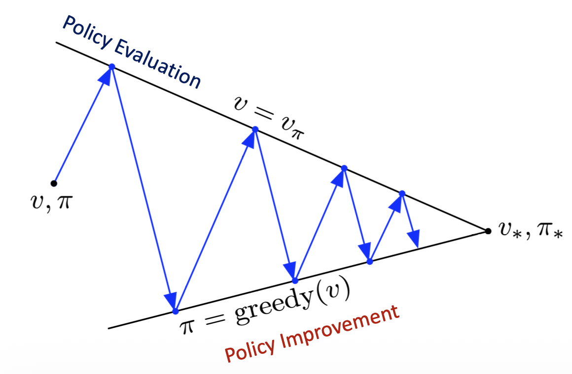
Policy Improvement​

  • π→vπ→π′\pi \to v_\pi \to \pi'
  • π′=greedy(vπ)\pi' = \text{greedy}(v_\pi)
  • Evaluate current policy, Improve it greedily, then get a better policy

Policy Improvement

Modified Policy Iteration​

  • Policy iteration can be computationally expensive
  • MPI: cut off the policy evaluation after a few iterations kk then step to policy improvement.
    • k=1⇒Value iterationk = 1 \Rightarrow \text{Value iteration}
    • k=3,4⇒Modified Policy iterationk = 3,4 \Rightarrow \text{Modified Policy iteration}
    • kis large enough⇒Policy iterationk \quad \text{is large enough} \Rightarrow \text{Policy iteration}

Poisson Distribution Formulation​

P(X=n)=λne−λn!P(X = n) = \frac{\lambda^n e^{-\lambda}}{n!}

  • How many times an event occurs within a fixed interval of time (or space) when we only know the long-term average rate (λ\lambda).
  • nn: The actual number of requests or returns (n∈{0,1,2,…}n \in \{0, 1, 2, \ldots\})
  • λ\lambda: The expected/average number of requests or returns
  • ee: Euler's number (2.71828)
  • n!n!: Factorial of nn

Deterministic Value Iteration​

v∗(s)=max⁡a(R(s,a)+γ∑s′P(s′∣s,a)v∗(s′))v_*(s) = \max_{a} \left( \mathcal{R}(s,a) + \gamma \sum_{s'} P(s'|s,a) v_*(s') \right)

  • If solutions to sub-problems v∗(s′)v_*(s') are known, the optimal value v∗(s)v_*(s) for the current state can be computed directly.
  • Value signals propagate backwards across the state space from states with terminal rewards.

Value Iteration​

vk+1(s)=max⁡a(R(s,a)+γ∑s′P(s′∣s,a)vk(s′))v_{k+1}(s) = \max_{a} \left( \mathcal{R}(s,a) + \gamma \sum_{s'} P(s'|s,a) v_k(s') \right)

  • Infinite (∞\infty) iterations are required to converge exactly to v∗v_*.
  • In practical implementations, iteration terminates when the maximum value change between iterations is less than a small threshold θ\theta.

Dynamic Programming ALgorithms​

ProblemBellman EquationAlgorithm
PredictionBellman Expectation:
vk+1(s)=∑a∈Aπ(a∣s)(R(s,a)+γ∑s′∈SP(s′∣s,a)vk(s′))v_{k+1}(s) = \sum_{a \in A} \pi(a \mid s) \left( R(s, a) + \gamma \sum_{s' \in S} P(s' \mid s, a) v_k(s') \right)
Iterative Policy Evaluation
ControlBellman Expectation + Greedy Policy Improvement:
vk+1(s)=∑a∈Aπ(a∣s)(R(s,a)+γ∑s′∈SP(s′∣s,a)vk(s′))v_{k+1}(s) = \sum_{a \in A} \pi(a \mid s) \left( R(s, a) + \gamma \sum_{s' \in S} P(s' \mid s, a) v_k(s') \right)
π′=greedy(Vπ)\pi' = \text{greedy}(V_\pi)
Policy Iteration
ControlBellman Optimality:
vk+1(s)=max⁡a(R(s,a)+γ∑s′∈SP(s′∣s,a)vk(s′))v_{k+1}(s) = \max_a \left( R(s, a) + \gamma \sum_{s' \in S} P(s' \mid s, a) v_k(s') \right)
Value Iteration

Efficiency of DP​

  • Strengths:
    • A foundational and efficient framework widely used for solving MDPs.
    • Mathematically guaranteed to converge to an optimal policy in polynomial time in terms of the number of states and actions.
    • Exponentially faster than exhaustive direct search across the policy space (∣A∣∣S∣|A|^{|S|}).
  • Limitations:
    • Can become computationally impractical for extremely large or complex environments.
    • Curse of Dimensionality: As the number of state variables (dimensions) increases, the total state space size (∣S∣|S|) expands exponentially, leading to severe computational and memory bottlenecks.

Asynchronous Dynamic Programming​

  • Comparison with Synchronous Methods: Standard DP methods sweep through the entire state space systematically in every iteration. Asynchronous DP backs up individual states independently in arbitrary order.
  • In-place Value Updates: Directly overwrites values in a single memory array, allowing immediate propagation of newly updated state values to subsequent calculations.
  • Computational Gain & Convergence:
    • Significantly reduces computation by avoiding exhaustive full-state sweeps.
    • Guaranteed to converge to the optimal value function v∗v_*, provided that all states continue to be selected and updated indefinitely.

Real-Time Dynamic Programming (RTDP)​

  • Interaction-Driven Online Updates: Solves sub-problems on-the-fly by focusing updates specifically on states that are directly relevant to the agent's current trajectory.
  • Target Applications: Large-scale environments where full state-space iteration is intractable (e.g., robotics, autonomous control systems, game AI).
  • Core Characteristics:
    • Online Decision Making: Makes and refines decisions while operating directly in the environment.
    • Lazy Evaluation: Computes values only for visited or critical state subsets rather than unvisited distant states.
    • Adaptive Exploration: Guides search toward high-reward trajectories through active interaction.
    • Approximate MDP Solution: Yields near-optimal policies for relevant regions without solving the global MDP.

Approximate Dynamic Programming (ADP)​

  • Motivation: Addresses the curse of dimensionality where tabular representation of states and exact value computation become computationally infeasible.
  • Function Approximation Methods: Parameterizes and estimates the value function using scalable statistical and machine learning models:
    • Linear models, deep neural networks, decision trees, and general regression techniques.
  • Error Management Mechanisms:
    • Eligibility Traces: Accelerates credit assignment and temporal consistency across multi-step transitions.
    • Experience Replay: Stores transition tuples in a replay buffer and samples them randomly to break data correlation and stabilize value approximation.

RL 004

· 약 16분

Bellman Equation​

vπ(s)=Eπ[Rt+1⏟Immediate Reward+γvπ(St+1)⏟Discounted Future Value  |  St=s⏟Starting at state s]v_\pi(s) = \mathbb{E}_\pi \left[ \underbrace{R_{t+1}}_{\text{Immediate Reward}} + \gamma \underbrace{v_\pi(S_{t+1})}_{\text{Discounted Future Value}} \;\middle|\; \underbrace{S_t = s}_{\text{Starting at state s}} \right]

  • Fundamental concept in RL using a recursive equation to express a way to compute the value of a state based on the values of its successor states.
v(s)=E[Rt+1+γRt+2+γ2Rt+3+…  |  St=s]=E[Rt+1+γ(Rt+2+γRt+3+… )⏟Gt+1  |  St=s]=E[Rt+1+γGt+1  |  St=s]=E[Rt+1+γv(St+1)  |  St=s]=E[Rt+1∣St=s]⏟Immediate Reward R(s)+γ E[v(St+1)∣St=s]⏟Expected Next State Value(∵E[X+γY]=E[X]+γE[Y])=R(s)+γ∑s′P(s′∣s)v(s′)⏟Transition Dynamics(∵E[g(X)]=∑xP(x)g(x))\begin{aligned} v(s) &= \mathbb{E} \left[ R_{t+1} + \gamma R_{t+2} + \gamma^2 R_{t+3} + \dots \;\middle|\; S_t = s \right] \\[8pt] &= \mathbb{E} \left[ R_{t+1} + \gamma \underbrace{\left( R_{t+2} + \gamma R_{t+3} + \dots \right)}_{G_{t+1}} \;\middle|\; S_t = s \right] \\[8pt] &= \mathbb{E} \left[ R_{t+1} + \gamma G_{t+1} \;\middle|\; S_t = s \right] \\[8pt] &= \mathbb{E} \left[ R_{t+1} + \gamma v(S_{t+1}) \;\middle|\; S_t = s \right] \\[8pt] &= \underbrace{\mathbb{E}[R_{t+1} \mid S_t = s]}_{\text{Immediate Reward } \mathcal{R}(s)} + \gamma \, \underbrace{\mathbb{E}[v(S_{t+1}) \mid S_t = s]}_{\text{Expected Next State Value}} && (\because \mathbb{E}[X + \gamma Y] = \mathbb{E}[X] + \gamma\mathbb{E}[Y]) \\[10pt] &= \mathcal{R}(s) + \gamma \underbrace{\sum_{s'} \mathcal{P}(s' \mid s) v(s')}_{\text{Transition Dynamics}} && \left(\because \mathbb{E}[g(X)] = \sum_x P(x)g(x)\right) \end{aligned}

Bellman Equation Example​

Bellman Example

v(sBL)=7+γ(0.1⋅v(sBL)+0.5⋅(sTL)+0.4⋅(sBR))v(s_{\text{BL}}) = 7 + \gamma(0.1 \cdot v(s_{\text{BL}}) + 0.5 \cdot(s_{TL}) + 0.4 \cdot(s_{BR}))

Bellman Equation in Matrix Form​

v=R+γPvv = \mathcal{R} + \gamma \mathcal{P} v

[v(s1)⋮v(sn)]⏟V of a particular state=[R(s1)⋮R(sn)]⏟Immediate Reward+γ[P11⋯P1n⋮⋱⋮Pn1⋯Pnn]⏟Transition Matrix[v(s1)⋮v(sn)]⏟V of future state\begin{aligned} \underbrace{ \begin{bmatrix} v(s_1) \\ \vdots \\ v(s_n) \end{bmatrix}}_{\text{V of a particular state}} = \underbrace{\begin{bmatrix} \mathcal{R}(s_1) \\ \vdots \\ \mathcal{R}(s_n) \end{bmatrix}}_{\text{Immediate Reward}} + \gamma \underbrace{\begin{bmatrix} \mathcal{P}_{11} & \cdots & \mathcal{P}_{1n} \\ \vdots & \ddots & \vdots \\ \mathcal{P}_{n1} & \cdots & \mathcal{P}_{nn} \end{bmatrix}}_{\text{Transition Matrix}} \underbrace{\begin{bmatrix} v(s_1) \\ \vdots \\ v(s_n) \end{bmatrix}}_{\text{V of future state}} \end{aligned}

Solving the Bellman Equation​

Linear System of Equations​

v=R+γPvv−γPv=R(I−γP)v=Rv=(I−γP)−1R\begin{aligned} \mathcal{v} &= \mathcal{R} + \gamma \mathcal{P}\mathcal{v} \\ \mathcal{v} - \gamma \mathcal{P}\mathcal{v} &= \mathcal{R} \\ (I - \gamma \mathcal{P})\mathcal{v} &= \mathcal{R} \\ \mathcal{v} &= (I - \gamma \mathcal{P})^{-1} \mathcal{R} \end{aligned}
  • Computational Complexity: O(n3)O(n^3)
  • For small MDPs: direct solution is possible (up to 100 states)
  • For large MDPs:
    • Iterative methods
    • Dynamic Programming
    • Monte Carlo Tree
    • TD learning

State-Value Function​

vπ(s)⏟Value of state s=Eπ⏟Follows policy π[Rt+1⏟Immediate Reward+γvπ(St+1)⏟Discounted Value of Next State  |  St=s⏟Starting at state s]\begin{aligned} \underbrace{v_\pi(s)}_{\text{Value of state } s} = \underbrace{\mathbb{E}_\pi}_{\text{Follows policy } \pi} \left[ \underbrace{R_{t+1}}_{\text{Immediate Reward}} + \gamma \underbrace{v_\pi(S_{t+1})}_{\text{Discounted Value of Next State}} \;\middle|\; \underbrace{S_t = s}_{\text{Starting at state } s} \right] \end{aligned}
  • Evaluates the expected return starting from state ss and following policy π\pi thereafter.
  • How good is it to be in state ss?
  • vπ(s)v_\pi(s): Expected cumulative return starting from state ss under policy π\pi.
  • Eπ\mathbb{E}_\pi: Expectation over action selections (At∼πA_t \sim \pi) and transition dynamics (St+1∼PS_{t+1} \sim \mathcal{P}).
  • Rt+1R_{t+1}: Immediate reward received upon transitioning out of state ss.
  • γvπ(St+1)\gamma v_\pi(S_{t+1}): Discounted expected value of the next successor state St+1S_{t+1}.
  • St=sS_t = s: Condition that the agent starts at state ss at time step tt.

vπ(s)=∑a∈Aπ(a∣s)qπ(s,a)v_{\pi}(s) = \sum_{a \in \mathcal{A}} \pi(a \mid s) q_{\pi}(s, a)

  • The value of state ss is the policy-weighted average of the values of all possible actions that can be taken from that state.
  • vπ(s)v_{\pi}(s): Expected cumulative return starting from state ss under policy π\pi.
  • π(a∣s)\pi(a \mid s): Probability of taking action aa in state ss under policy π\pi.
  • qπ(s,a)q_{\pi}(s, a): Value of taking action aa in state ss under policy π\pi.

Action-Value Function​

qπ(s,a)⏟Action-Value of (s,a)=Eπ⏟Follows policy π[Rt+1⏟Immediate Reward+γqπ(St+1,At+1)⏟Discounted Next Action-Value  |  St=s,At=a⏟Starting at s taking action a]\begin{aligned} \underbrace{q_\pi(s, a)}_{\text{Action-Value of } (s, a)} = \underbrace{\mathbb{E}_\pi}_{\text{Follows policy } \pi} \left[ \underbrace{R_{t+1}}_{\text{Immediate Reward}} + \gamma \underbrace{q_\pi(S_{t+1}, A_{t+1})}_{\text{Discounted Next Action-Value}} \;\middle|\; \underbrace{S_t = s, A_t = a}_{\text{Starting at } s \text{ taking action } a} \right] \end{aligned}
  • Evaluates the expected return of taking an arbitrary action aa in state ss, and subsequently following policy π\pi from step t+1t+1 onward.
  • How good is it to take action aa in state ss?
  • qπ(s,a)q_\pi(s, a): Value of taking action aa in state ss under policy π\pi (Q-value).
  • Eπ\mathbb{E}_\pi: Expectation over the next transition (St+1∼PS_{t+1} \sim \mathcal{P}) and the subsequent action (At+1∼πA_{t+1} \sim \pi).
  • Rt+1R_{t+1}: Immediate reward resulting from the state-action pair (s,a)(s, a).
  • γqπ(St+1,At+1)\gamma q_\pi(S_{t+1}, A_{t+1}): Discounted expected value of the successor state-action pair (St+1,At+1)(S_{t+1}, A_{t+1}).
  • St=s,At=aS_t = s, A_t = a: Condition that both the initial state and the initial action are fixed at time tt.
vπ(s)=∑a∈Aπ(a∣s)(Rsa+γ∑s′∈SPss′avπ(s′))\begin{aligned} v_\pi(s) = \sum_{a \in \mathcal{A}} \pi(a \mid s) \left( \mathcal{R}_s^a + \gamma \sum_{s' \in \mathcal{S}} \mathcal{P}_{ss'}^a v_\pi(s') \right) \end{aligned}
  • Evaluates state ss directly by averaging over all possible action branches (π\pi) and their subsequent environmental transitions (P\mathcal{P}).
  • Rsa\mathcal{R}_s^a: Immediate reward resulting from the state-action pair (s,a)(s, a).
  • γ∑s′∈SPss′avπ(s′)\gamma \sum_{s' \in \mathcal{S}} \mathcal{P}_{ss'}^a v_\pi(s'): Discounted expected value of the successor state s′s' resulting from the state-action pair (s,a)(s, a).
  • Pss′a\mathcal{P}_{ss'}^a: Probability of transitioning from state ss to state s′s' when action aa is taken.
  • S\mathcal{S}: Set of all possible states.
  • A\mathcal{A}: Set of all possible actions.
  • π(a∣s)\pi(a \mid s): Probability of taking action aa in state ss under policy π\pi.
  • vπ(s′)v_\pi(s'): Value of state s′s' under policy π\pi.

Bellman Expectation Equation​

qπ(s,a)=Rsa+γ∑s′∈SPss′a∑a′∈Aπ(a′∣s′)qπ(s′,a′)\begin{aligned} q_\pi(s, a) = \mathcal{R}_s^a + \gamma \sum_{s' \in \mathcal{S}} \mathcal{P}_{ss'}^a \sum_{a' \in \mathcal{A}} \pi(a' \mid s') q_\pi(s', a') \end{aligned}
  • Evaluates the state-action pair (s,a)(s, a) by summing immediate reward and the expected value of future action pairs (s′,a′)(s', a'), averaged across transition dynamics P\mathcal{P} and next-step policy choices π\pi.
  • Rsa\mathcal{R}_s^a: Immediate reward resulting from the state-action pair (s,a)(s, a).
  • γ∑s′∈SPss′a∑a′∈Aπ(a′∣s′)qπ(s′,a′)\gamma \sum_{s' \in \mathcal{S}} \mathcal{P}_{ss'}^a \sum_{a' \in \mathcal{A}} \pi(a' \mid s') q_\pi(s', a'): Discounted expected value of the successor state-action pair (s′,a′)(s', a') resulting from the state-action pair (s,a)(s, a).
  • Pss′a\mathcal{P}_{ss'}^a: Probability of transitioning from state ss to state s′s' when action aa is taken.
  • S\mathcal{S}: Set of all possible states.
  • A\mathcal{A}: Set of all possible actions.
  • π(a′∣s′)\pi(a' \mid s'): Probability of taking action a′a' in state s′s' under policy π\pi.
vπ(s)→Action Policy πqπ(s,a)↑↓Environment Transition Pvπ(s′)←Environment Transition Pqπ(s′,a′)\begin{matrix} v_\pi(s) & \xrightarrow{\text{Action Policy } \pi} & q_\pi(s, a) \\ \uparrow & & \downarrow \text{Environment Transition } \mathcal{P} \\ v_\pi(s') & \xleftarrow{\text{Environment Transition } \mathcal{P}} & q_\pi(s', a') \end{matrix}

Optimal Value Function​

V∗(s)=max⁡πvπ(s)V_*(s) = \max_\pi v_\pi(s)

  • The optimal State-Value Function V∗(s)V_*(s)
  • Maximum value function over all policies, or maximum possible reward that can be achieved from state ss.

q∗(s,a)=max⁡πqπ(s,a)q_*(s, a) = \max_\pi q_\pi(s, a)

  • The Optimal Action-Value Function q∗(s,a)q_*(s, a)
  • Maximum action-value function over all policies, or given state ss and action taken aa, what is the maximum reward that can be achieved from there onwards.

Optimal Policy​

π∗≥π  ⟺  vπ∗(s)≥vπ(s)∀s∈S\pi_* \geq \pi \iff v_{\pi_*(s)} \geq v_\pi(s) \quad \forall s \in \mathcal{S}

  • If certain policy is better than another policy, then the value of the better policy is greater than or equal to the value of others in all states.

Theorem fo any MDP​

  • Existence of an Optimal Policy: There always exists at least one optimal policy π∗\pi_* that is better than or equal to all other policies across all states (π∗≥π,  ∀π\pi_* \ge \pi, \; \forall \pi).
  • Uniqueness of the Optimal State-Value Function: Although multiple distinct optimal policies may exist (e.g., when two different paths yield the exact same maximum expected return), all optimal policies achieve the exact same unique optimal state-value function (vπ∗(s)=v∗(s)v_{\pi_*}(s) = v_*(s)).
  • Uniqueness of the Optimal Action-Value Function: Similarly, all optimal policies achieve the exact same unique optimal action-value function (qπ∗(s,a)=q∗(s,a)q_{\pi_*}(s, a) = q_*(s, a)).

Finding an Optimal Policy​

π∗(a∣s)={1if a=arg⁡max⁡a∈Aq∗(s,a)0otherwise\pi_*(a \mid s) = \begin{cases} 1 & \text{if } a = \arg\max_{a \in \mathcal{A}} q_*(s, a) \\ 0 & \text{otherwise} \end{cases}
  • If q∗(s,a)q_*(s, a) is known, optimal policy is achieved.
  • A deterministic optimal policy always exists for any MDP.

Bellman Optimality Equation​

Bellman Optimality Equation for v∗v_*​

v∗(s)⏟Optimal Value of State s=max⁡a∈Aq∗(s,a)⏟Optimal Value of Action a\begin{aligned} \underbrace{v_*(s)}_{\text{Optimal Value of State } s} = \max_{a \in \mathcal{A}} \underbrace{q_*(s, a)}_{\text{Optimal Value of Action } a} \end{aligned}
  • State-Value to Action-Value (s→as \rightarrow a)
  • The optimal state-value is achieved by greedily picking the single action that yields the maximum optimal action-value.
q∗(s,a)⏟Optimal Action-Value=Rsa⏟Immediate Reward+γ∑s′∈SPss′av∗(s′)⏟Expected Optimal Future Value\begin{aligned} \underbrace{q_*(s, a)}_{\text{Optimal Action-Value}} = \underbrace{\mathcal{R}_s^a}_{\text{Immediate Reward}} + \gamma \underbrace{\sum_{s' \in \mathcal{S}} \mathcal{P}_{ss'}^a v_*(s')}_{\text{Expected Optimal Future Value}} \end{aligned}
  • Action-Value to Next State-Value (a→s′a \rightarrow s')
  • Once the action aa is committed, the outcome is governed by the environment dynamics Pss′a\mathcal{P}_{ss'}^a, requiring an expectation (average) over possible successor states s′s'.
v∗(s)⏟Optimal Value of State s=max⁡a∈A(Rsa⏟Immediate Reward+γ∑s′∈SPss′av∗(s′)⏟Expected Optimal Future Value)\begin{aligned} \underbrace{v_*(s)}_{\text{Optimal Value of State } s} = \max_{a \in \mathcal{A}} \left( \underbrace{\mathcal{R}_s^a}_{\text{Immediate Reward}} + \gamma \underbrace{\sum_{s' \in \mathcal{S}} \mathcal{P}_{ss'}^a v_*(s')}_{\text{Expected Optimal Future Value}} \right) \end{aligned}
  • Bellman Optimality Equation for v∗v_* (s→a→s′s \rightarrow a \rightarrow s')
  • Combines the agent's deterministic maximization (max⁡a\max_a) with the environment's stochastic transition (∑s′Pss′a\sum_{s'} \mathcal{P}_{ss'}^a).
    • It means a structure where the best choice I can make (max⁡\max) embeds the probabilistic outcomes of the world (∑\sum) in its calculation.
  • Non-Linear System: Because of the max⁡\max operator, this system of equations cannot be solved directly via matrix inversion (I−γP)−1(I - \gamma\mathcal{P})^{-1}
    • it must be solved iteratively via Dynamic Programming (Value Iteration) or Reinforcement Learning.

Bellman Optimality Equation for q∗q_*​

q∗(s,a)⏟Optimal Action-Value=Rsa⏟Immediate Reward+γ∑s′∈SPss′a⏟Transition Dynamicsmax⁡a′∈Aq∗(s′,a′)⏟Optimal Successor Action\begin{aligned} \underbrace{q_*(s, a)}_{\text{Optimal Action-Value}} = \underbrace{\mathcal{R}_s^a}_{\text{Immediate Reward}} + \gamma \underbrace{\sum_{s' \in \mathcal{S}} \mathcal{P}_{ss'}^a}_{\text{Transition Dynamics}} \underbrace{\max_{a' \in \mathcal{A}} q_*(s', a')}_{\text{Optimal Successor Action}} \end{aligned}
  • Bellman Optimality Equation for q∗q_* ((s,a)→s′→a′(s, a) \to s' \to a')
  • Action Commitment: The initial state ss and action aa are fixed, receiving immediate reward Rsa\mathcal{R}_s^a.
  • Stochastic Transition: The agent transitions to successor state s′s' according to the environment's transition probability Pss′a\mathcal{P}_{ss'}^a.
  • Greedy Successor Action (max⁡a′\max_{a'}): Upon landing in state s′s', the agent greedily selects the action a′a' that yields the maximum possible optimal action-value q∗(s′,a′)q_*(s', a').
  • Core Foundation of Q-Learning: This equation directly forms the update target for off-policy algorithms like Q-Learning and DQN

Solving Bellman optimality equation​

  • Non-Linear equation: The optimality equations embed the non-linear max⁡\max operator, they cannot be linearized into standard matrix inversions.

Dynamic Programming Approaches​

πk+1(s)=arg⁡max⁡a∈A[Rsa+γ∑s′∈SPss′avπk(s′)]\begin{aligned} \pi_{k+1}(s) = \arg\max_{a \in \mathcal{A}} \left[ \mathcal{R}_s^a + \gamma \sum_{s' \in \mathcal{S}} \mathcal{P}_{ss'}^a v_{\pi_k}(s') \right] \end{aligned}
  • Policy Iteration: Alternates between full Policy Evaluation and Policy Improvement until the policy stabilizes (πk+1=πk\pi_{k+1} = \pi_k).
vk+1(s)←max⁡a∈A[Rsa+γ∑s′∈SPss′avk(s′)]\begin{aligned} v_{k+1}(s) \leftarrow \max_{a \in \mathcal{A}} \left[ \mathcal{R}_s^a + \gamma \sum_{s' \in \mathcal{S}} \mathcal{P}_{ss'}^a v_k(s') \right] \end{aligned}
  • Value Iteration: Turns the Bellman Optimality Equation directly into an iterative update rule, bypassing explicit policy evaluation steps.

Temporal-Difference Control Approaches​

Q(St,At)←Q(St,At)+α[Rt+1+γmax⁡aQ(St+1,a)⏟Off-policy Target from q∗−Q(St,At)]\begin{aligned} Q(S_t, A_t) \leftarrow Q(S_t, A_t) + \alpha \left[ \underbrace{R_{t+1} + \gamma \max_{a} Q(S_{t+1}, a)}_{\text{Off-policy Target from } q_*} - Q(S_t, A_t) \right] \end{aligned}
  • Q-Learning (Off-Policy TD Control): Learns optimal action-values q∗q_* directly from experience tuples (St,At,Rt+1,St+1)(S_t, A_t, R_{t+1}, S_{t+1}) by approximating the Bellman Optimality Equation via bootstrapping.
Q(St,At)←Q(St,At)+α[Rt+1+γQ(St+1,At+1)⏟On-policy Target from qπ−Q(St,At)]\begin{aligned} Q(S_t, A_t) \leftarrow Q(S_t, A_t) + \alpha \left[ \underbrace{R_{t+1} + \gamma Q(S_{t+1}, A_{t+1})}_{\text{On-policy Target from } q_\pi} - Q(S_t, A_t) \right] \end{aligned}
  • SARSA (On-Policy TD Control): Learns action-values qπq_\pi for the current policy from experience transitions (St,At,Rt+1,St+1,At+1)(S_t, A_t, R_{t+1}, S_{t+1}, A_{t+1}), steadily improving the policy toward optimality.

Policy Evaluation​

  • Evaluate a given policy π\pi is a prediction problem.
  • Iterative application of Bellman Expectation backup.
Input:π:Policy to be evaluatedParameters:θ>0:Small threshold determining estimation accuracyγ∈[0,1]:Discount factorInitialize:V(s)∈R,∀s∈SV(terminal)=0Repeat:Δ←0For each s∈S:v←V(s)V(s)←∑a∈Aπ(a∣s)(Rsa+γ∑s′∈SPss′aV(s′))Δ←max⁡(Δ,  ∣v−V(s)∣)Until Δ<θOutput:V≈vπ\begin{aligned} &\textbf{Input:} \\ &\quad \pi : \text{Policy to be evaluated} \\[6pt] &\textbf{Parameters:} \\ &\quad \theta > 0 : \text{Small threshold determining estimation accuracy} \\ &\quad \gamma \in [0, 1] : \text{Discount factor} \\[6pt] &\textbf{Initialize:} \\ &\quad V(s) \in \mathbb{R}, \quad \forall s \in \mathcal{S} \\ &\quad V(\text{terminal}) = 0 \\[8pt] &\textbf{Repeat:} \\ &\quad \Delta \leftarrow 0 \\ &\quad \textbf{For each } s \in \mathcal{S}: \\ &\quad\quad v \leftarrow V(s) \\ &\quad\quad V(s) \leftarrow \sum_{a \in \mathcal{A}} \pi(a \mid s) \left( \mathcal{R}_s^a + \gamma \sum_{s' \in \mathcal{S}} \mathcal{P}_{ss'}^a V(s') \right) \\ &\quad\quad \Delta \leftarrow \max \left( \Delta, \; |v - V(s)| \right) \\ &\textbf{Until } \Delta < \theta \\[8pt] &\textbf{Output:} \\ &\quad V \approx v_\pi \end{aligned}
  • π\pi: Target policy being evaluated (π(a∣s)\pi(a \mid s) is the action selection probability).
  • θ\theta: Small threshold (θ>0\theta > 0) defining the stopping criterion for convergence.
  • γ\gamma: Discount factor (γ∈[0,1]\gamma \in [0, 1]) for future rewards.
  • V(s)V(s): Current estimated value of state ss (with V(terminal)=0V(\text{terminal}) = 0).
  • Δ\Delta: Maximum absolute value change across all states during the current sweep (max⁡∣v−V(s)∣\max |v - V(s)|).
  • Rsa\mathcal{R}_s^a: Expected immediate reward from taking action aa in state ss.
  • Pss′a\mathcal{P}_{ss'}^a: Transition probability to successor state s′s' from state ss via action aa.
  • vπv_\pi: True state-value function under policy π\pi that V(s)V(s) converges to.

Policy Improvement​

π′(s)=arg⁡max⁡a∈A[Rsa+γ∑s′∈SPss′aVπ(s′)]⏟qπ(s,a)\begin{aligned} \pi'(s) = \arg\max_{a \in \mathcal{A}} \underbrace{\left[ \mathcal{R}_s^a + \gamma \sum_{s' \in \mathcal{S}} \mathcal{P}_{ss'}^a V_\pi(s') \right]}_{q_\pi(s, a)} \end{aligned}
  • Computing Value-function for a policy helps to find better policies.
  • Evaluate the policy π\pi, find Vπ(s)V_\pi(s)
  • Improve the policy by greedy action: π′=greedy(Vπ)\pi' = \text{greedy}(V_\pi)
  • π\pi: Current baseline policy before improvement.
  • Vπ(s)V_\pi(s): True state-value function evaluated under policy π\pi.
  • π′\pi': New, improved policy updated via greedy action selection.
  • arg⁡max⁡a\arg\max_{a}: The operation of selecting the action aa that maximizes the subsequent expected return (qπ(s,a)q_\pi(s, a)).
  • Rsa\mathcal{R}_s^a: Immediate expected reward earned by taking action aa in state ss.
  • γ\gamma: Discount factor (γ∈[0,1]\gamma \in [0, 1]).
  • Pss′a\mathcal{P}_{ss'}^a: Transition probability to successor state s′s' from state ss via action aa.

Policy Iteration Algorithm​

Policy Iteration = Evaluate -> Improve -> Repeat

1. InitializationV(s)∈R and π(s)∈A(s) arbitrarily for all s∈S2. Policy EvaluationLoop:Δ←0Loop for each s∈S:v←V(s)V(s)←∑s′,rp(s′,r∣s,π(s))[r+γV(s′)]Δ←max⁡(Δ,  ∣v−V(s)∣)until Δ<θ(θ>0, small positive threshold)3. Policy Improvementpolicy-stable←trueFor each s∈S:old-action←π(s)π(s)←arg⁡max⁡a∈A(s)∑s′,rp(s′,r∣s,a)[r+γV(s′)]if old-action≠π(s) then policy-stable←falseif policy-stable then stop and return V≈v∗ and π≈π∗else go to 2\begin{aligned} &\textbf{1. Initialization} \\ &\quad V(s) \in \mathbb{R} \text{ and } \pi(s) \in \mathcal{A}(s) \text{ arbitrarily for all } s \in \mathcal{S} \\[6pt] &\textbf{2. Policy Evaluation} \\ &\quad \textbf{Loop:} \\ &\quad\quad \Delta \leftarrow 0 \\ &\quad\quad \textbf{Loop for each } s \in \mathcal{S}: \\ &\quad\quad\quad v \leftarrow V(s) \\ &\quad\quad\quad V(s) \leftarrow \sum_{s', r} p(s', r \mid s, \pi(s)) \left[ r + \gamma V(s') \right] \\ &\quad\quad\quad \Delta \leftarrow \max \left( \Delta, \; |v - V(s)| \right) \\ &\quad \textbf{until } \Delta < \theta \quad \text{($\theta > 0$, small positive threshold)} \\[6pt] &\textbf{3. Policy Improvement} \\ &\quad \textit{policy-stable} \leftarrow \text{true} \\ &\quad \textbf{For each } s \in \mathcal{S}: \\ &\quad\quad \textit{old-action} \leftarrow \pi(s) \\ &\quad\quad \pi(s) \leftarrow \arg\max_{a \in \mathcal{A}(s)} \sum_{s', r} p(s', r \mid s, a) \left[ r + \gamma V(s') \right] \\ &\quad\quad \textbf{if } \textit{old-action} \neq \pi(s) \textbf{ then } \textit{policy-stable} \leftarrow \text{false} \\[4pt] &\quad \textbf{if } \textit{policy-stable} \textbf{ then stop and return } V \approx v_* \text{ and } \pi \approx \pi_* \\ &\quad \textbf{else go to 2} \end{aligned}
  • Policy Evaluation (Prediction): What happens if I follow this policy?
  • Vπ(s)V_\pi(s): How good is each state?
  • Qπ(s,a)Q_\pi(s,a): What happens if I take an action aa?
  • Policy Improvement: Which action is better?
  • Optimal Policy: Repeat until no change

Value function diagram

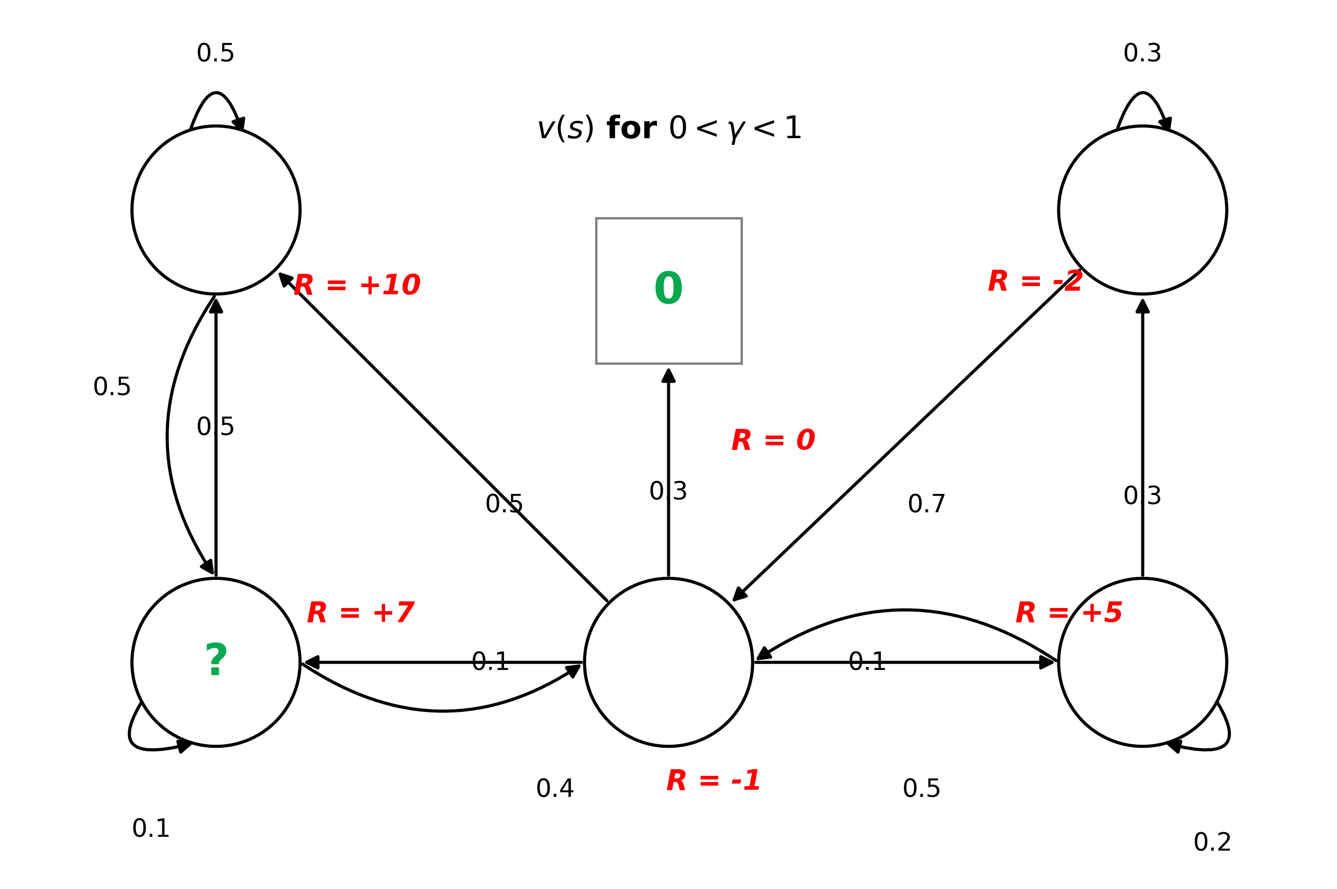
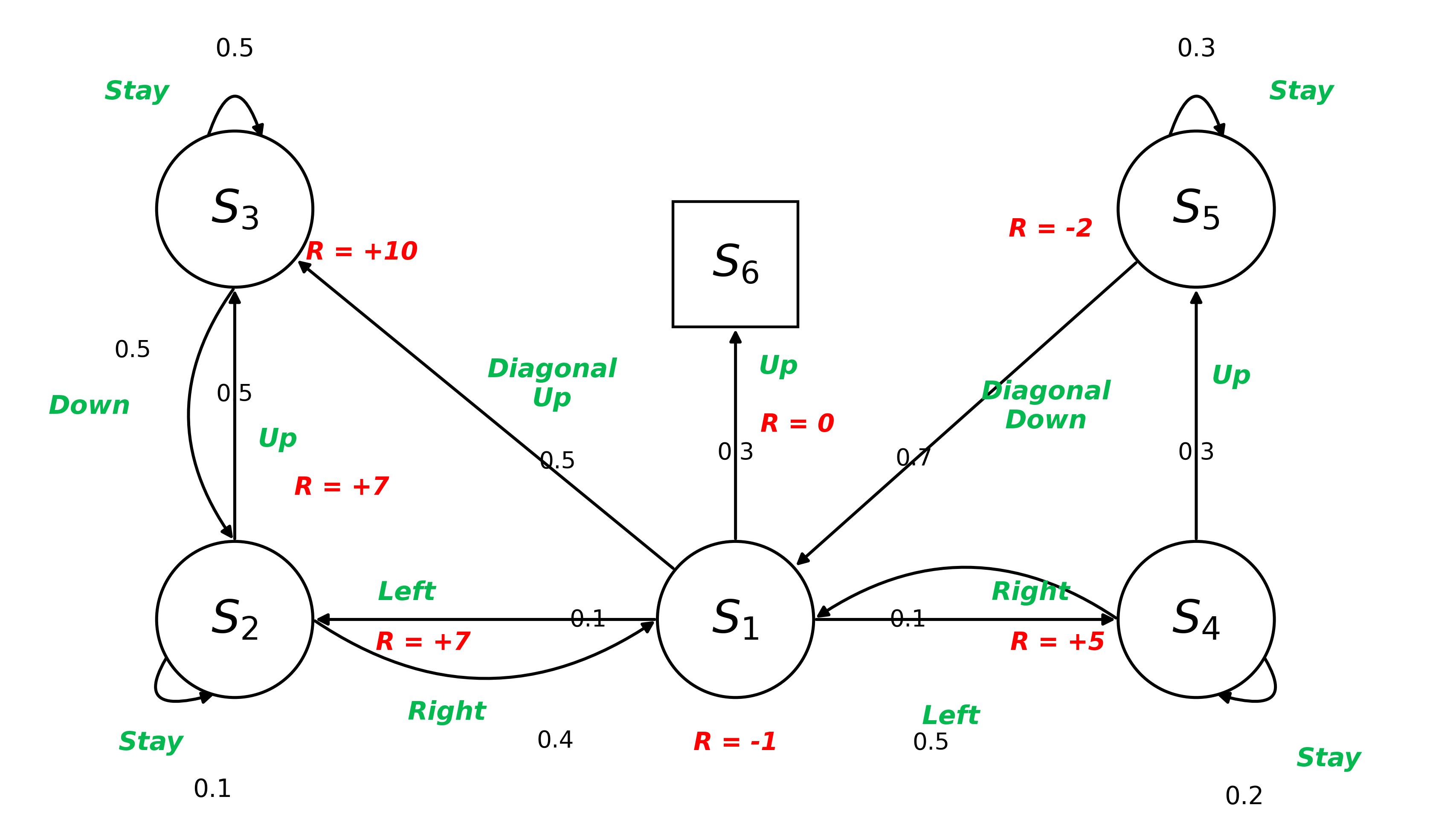
  • R(s1)=0.5(+10)+0.1(+7)+0.1(+5)+0.3(0)=6.2\mathcal{R}(s_1) = 0.5(+10) + 0.1(+7) + 0.1(+5) + 0.3(0) = \mathbf{6.2}
  • R(s2)=0.5(0)+0.1(0)+0.4(−1)=−0.4\mathcal{R}(s_2) = 0.5(0) + 0.1(0) + 0.4(-1) = \mathbf{-0.4}
  • R(s3)=0.5(0)+0.5(0)=0\mathcal{R}(s_3) = 0.5(0) + 0.5(0) = \mathbf{0}
  • R(s4)=0.3(0)+0.2(0)+0.5(0)=0\mathcal{R}(s_4) = 0.3(0) + 0.2(0) + 0.5(0) = \mathbf{0}
  • R(s5)=0.3(0)+0.7(−2)=−1.4\mathcal{R}(s_5) = 0.3(0) + 0.7(-2) = \mathbf{-1.4}
v(s1)=6.2+γ[0.1v(s2)+0.5v(s3)+0.1v(s4)](∵v(s6)=0)v(s2)=−0.4+γ[0.4v(s1)+0.1v(s2)+0.5v(s3)]v(s3)=0+γ[0.5v(s2)+0.5v(s3)]v(s4)=0+γ[0.5v(s1)+0.2v(s4)+0.3v(s5)]v(s5)=−1.4+γ[0.7v(s1)+0.3v(s5)]\begin{aligned} v(s_1) &= 6.2 + \gamma \left[ 0.1 v(s_2) + 0.5 v(s_3) + 0.1 v(s_4) \right] \quad (\because v(s_6) = 0) \\ v(s_2) &= -0.4 + \gamma \left[ 0.4 v(s_1) + 0.1 v(s_2) + 0.5 v(s_3) \right] \\ v(s_3) &= 0 + \gamma \left[ 0.5 v(s_2) + 0.5 v(s_3) \right] \\ v(s_4) &= 0 + \gamma \left[ 0.5 v(s_1) + 0.2 v(s_4) + 0.3 v(s_5) \right] \\ v(s_5) &= -1.4 + \gamma \left[ 0.7 v(s_1) + 0.3 v(s_5) \right] \end{aligned} [v(s1)v(s2)v(s3)v(s4)v(s5)]=(I−γ[00.10.50.100.40.10.50000.50.5000.5000.20.30.70000.3])−1[6.2−0.400−1.4]\begin{bmatrix} v(s_1) \\ v(s_2) \\ v(s_3) \\ v(s_4) \\ v(s_5) \end{bmatrix} = \left( \mathbf{I} - \gamma \begin{bmatrix} 0 & 0.1 & 0.5 & 0.1 & 0 \\ 0.4 & 0.1 & 0.5 & 0 & 0 \\ 0 & 0.5 & 0.5 & 0 & 0 \\ 0.5 & 0 & 0 & 0.2 & 0.3 \\ 0.7 & 0 & 0 & 0 & 0.3 \end{bmatrix} \right)^{-1} \begin{bmatrix} 6.2 \\ -0.4 \\ 0 \\ 0 \\ -1.4 \end{bmatrix}

v(s2)[1−0.1γ−0.5γ22−γ]=−0.4+0.4γv(s1)v(s_2) \left[ 1 - 0.1\gamma - \frac{0.5\gamma^2}{2 - \gamma} \right] = -0.4 + 0.4\gamma v(s_1)

RL 003

· 약 10분

Markov Property​

  • The future is independent of the past given the present state.
  • The current state is sufficient to determine the future, without history.

Markov State​

P[St+1∣St]=P[St+1=s′∣St=s]P[S_{t+1} | S_t] = P[S_{t+1} = s' | S_t = s]

  • tt: Time step
  • St+1S_{t+1}: Next state
  • StS_t: Current state
  • S1,…,StS_1, \ldots, S_t: History (All previous states)

State Transition Probability​

Pss′=P[St+1=s′∣St=s]P_{ss'} = P[S_{t+1} = s' | S_t = s]

  • Likelihood or probability of moving from one state ss to another state s′s' in the next time step t+1t+1.
  • ss: Markov State
  • s′s': Successor State
  • tt: Time step
  • State transition matrix PP defines the transitions probabilities between all states ss to all successor states s′s'.

State Transition Matrix​

P=s1…sn←(to state)s1⋮sn[P11…P1n⋮⋱⋮Pn1…Pnn]↑(from state)\mathcal{P} = \begin{array}{rl} & \begin{matrix} \textcolor{red}{\boldsymbol{s_1}} & \textcolor{red}{\boldsymbol{\dots}} & \textcolor{red}{\boldsymbol{s_n}} \end{matrix} \quad \leftarrow \text{(to state)} \\ \begin{matrix} \textcolor{red}{\boldsymbol{s_1}} \\ \textcolor{red}{\boldsymbol{\vdots}} \\ \textcolor{red}{\boldsymbol{s_n}} \end{matrix} & \hspace{-10pt} \begin{bmatrix} \mathcal{P}_{11} & \dots & \mathcal{P}_{1n} \\ \vdots & \ddots & \vdots \\ \mathcal{P}_{n1} & \dots & \mathcal{P}_{nn} \end{bmatrix} \\ \begin{matrix} \uparrow \\[-2pt] \mathclap{\text{(from state)}} \end{matrix} & \end{array}
  • State transition matrix PP defines the transition probabilities between all states ss to all successor states s′s'.
  • Probability of moving from state sns_n to s1s_1 is Pn1\mathcal{P}_{n1}.

Math cal​

Reinforcement Learning and Math Major Symbols

  • P\mathcal{P}: Transition Probability Matrix
  • S\mathcal{S}: State Space
  • A\mathcal{A}: Action Space
  • R\mathcal{R}: Reward Function
  • L\mathcal{L}: Loss Function
  • N(μ,σ2)\mathcal{N}(\mu, \sigma^2): Normal Distribution
  • D\mathcal{D}: Dataset
  • H\mathcal{H}: Entropy / Hypothesis Space

Markov Process​

Markov Chain

  • What is going to be happened next?
  • it goes through a sequence of states overtime.
  • Stochastic Process: The next state St+1S_{t+1} is determined by the current state StS_t and the transition probability matrix PP that exhibits the Markov Property.
  • Current state is independent of the past states.
  • Memoryless: History of states leading up to the current state is not necessary to predict the next/future state.
  • MP: ⟨S,P⟩\langle\mathcal{S},\mathcal{P}\rangle, What states comes next?, Observer's Perspective.
  • MRP: ⟨S,P,R,γ⟩\langle\mathcal{S},\mathcal{P},\mathcal{R},\gamma\rangle, How good/How much reward is this state in the long run?, Evaluator's Perspective.
  • MDP: ⟨S,A,P,R,γ⟩\langle\mathcal{S},\mathcal{A},\mathcal{P},\mathcal{R},\gamma\rangle, What action should I take right now to maximize the long-term reward?, Decision Maker's Perspective.

Pss′=P[St+1=s′∣St=s]\mathcal{P}_{ss'} = P[S_{t+1} = s' | S_t = s]

  • SS: a finite set of states.
  • P\mathcal{P}: a state transition matrix, defines the transitions probabilities from all states ss to all successor states s′s'.
  • NO REWARD, NO ACTIONS.

Transition Diagram​

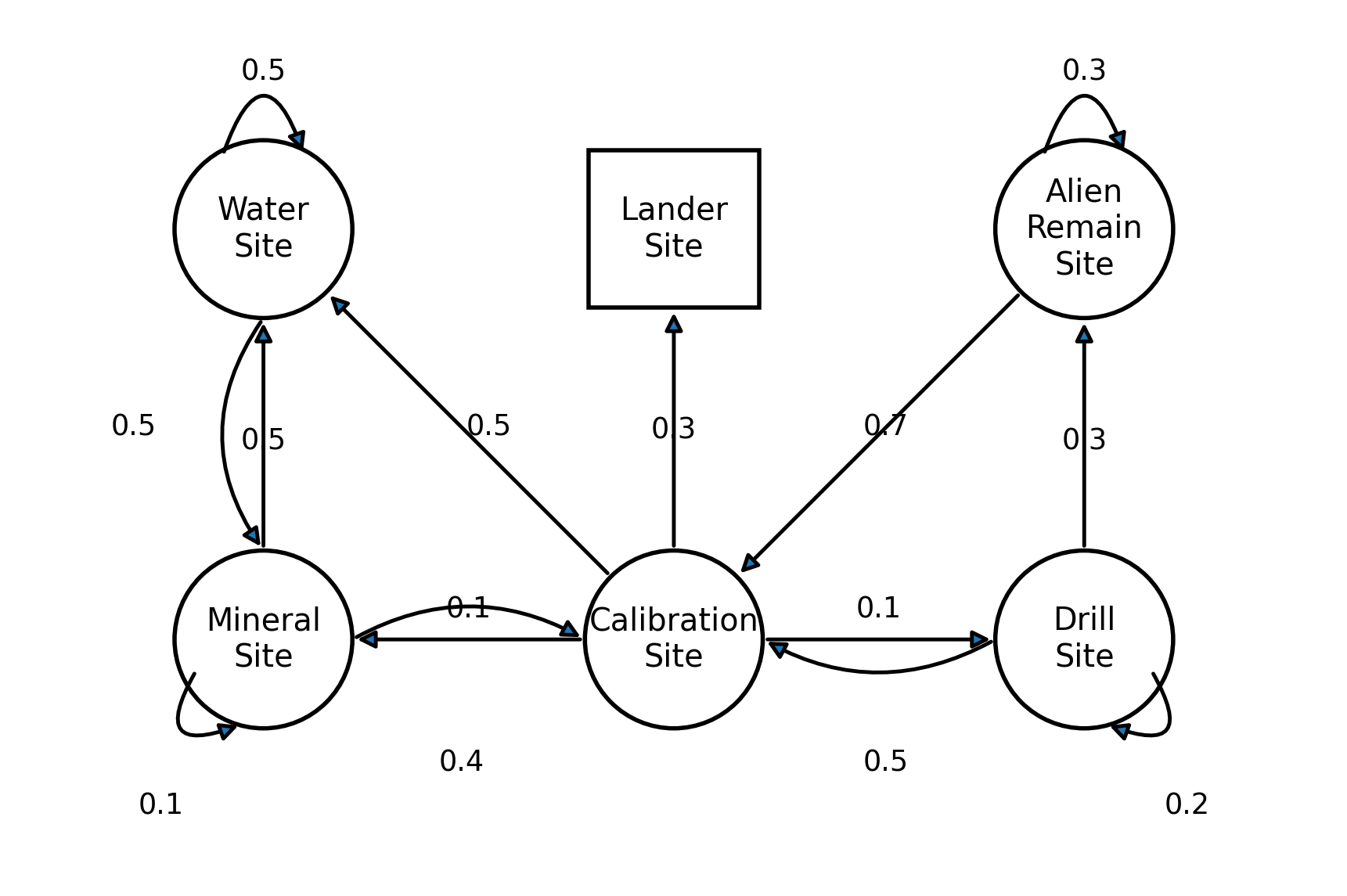
Moon Rover Transition Diagram

  • Box: where it ends
  • Arrow: transitions
  • Circle: states
  • Number: probability of transitioning to the state
P=[00.10.50.100.30.40.10.500000.50.50000.5000.20.300.70000.30000001]\mathcal{P} = \begin{bmatrix} 0 & 0.1 & 0.5 & 0.1 & 0 & 0.3 \\ 0.4 & 0.1 & 0.5 & 0 & 0 & 0 \\ 0 & 0.5 & 0.5 & 0 & 0 & 0 \\ 0.5 & 0 & 0 & 0.2 & 0.3 & 0 \\ 0.7 & 0 & 0 & 0 & 0.3 & 0 \\ 0 & 0 & 0 & 0 & 0 & 1 \end{bmatrix}
  • S1: Calibration Site
  • S2: Mineral Site
  • S3: Water Site
  • S4: Drill Site
  • S5: Alien Remain Site
  • S6: Lander Site

Markov Chain Episode​

  • A sequence of states from a starting state to a terminal state.
  • S1,S3,S2,S1,S6S_1, S_3, S_2, S_1, S_6
  • S1,S3,S3,S2,S1,S4,S4,S1,S6S_1, S_3, S_3, S_2, S_1, S_4, S_4, S_1, S_6

Episodic Task vs Continuous Task​

FeatureEpisodic TasksContinuing Tasks
TerminationHas a well-defined terminal state (TT)Runs indefinitely without termination (T=∞T = \infty)
Real-World Examples• Video games (e.g., Super Mario: level clear or death)
• Navigation (reaching destination)
• Board games (e.g., Chess: checkmate/draw)
• Smart thermostat (HVAC temperature control)
• 24/7 industrial robotic process control
• Automated trading & server load management
Execution FlowEnvironment resets to a start state once finishedOperates continuously without automatic resets
  • Episodic Tasks: Tasks with a defined end/terminal state.
  • Continuing Tasks: Tasks without a defined end/terminal state.
  • It may require different MDP formulation and solution methods for each type of task.

Markov Reward Process​

Markov Chain + Reward

⟨S,P,R,γ⟩\langle\mathcal{S},\mathcal{P},\mathcal{R},\gamma\rangle

  • SS: a finite set of states.
  • P\mathcal{P}: a state transition matrix (Transition Dynamics)
  • R\mathcal{R}: a reward function to compute expected reward from a state.
    • Rs=E[Rt+1∣St=s]\mathcal{R}_s = \mathbb{E}[R_{t+1} | S_t = s]
    • In the state ss, how much reward can you expect to get in the next time step?
  • γ\gamma: a discount factor, to balance the immediate and future rewards.
    • γ∈[0,1]\gamma \in [0, 1]

Reward diagram

Return​

Gt=Rt+1+Rt+2+⋯+RTG_t = R_{t+1} + R_{t+2} + \cdots + R_T

  • GtG_t: Goal Reward
    • The sum of the rewards received from time step tt.
  • Rt+1,Rt+2,…,RTR_{t+1}, R_{t+2}, \ldots, R_T: the sequence of rewards received after time step tt
  • TT: terminal state
  • tt: time step

Discount​

  • The present value of future rewards.
  • γ=0\gamma = 0: Myopic evaluation for maximizing immediate reward.
  • γ=1\gamma = 1: Far-sighted/Long-term evaluation for maximizing future reward.

Discounted Return​

Gt=Rt+1+γRt+2+γ2Rt+3+⋯+γT−t−1RT=∑k=0∞γkRt+k+1G_t = R_{t+1} + \gamma R_{t+2} + \gamma^2 R_{t+3} + \cdots + \gamma^{T-t-1} R_T = \sum_{k=0}^{\infty} \gamma^k R_{t+k+1}

  • GtG_t: Discounted Return
  • γ=1\gamma = 1: Undiscounted Markov Reward Process, if all sequences terminate (like games)

Value Function​

v(s)=E[Gt∣St=s]v(s) = \mathbb{E}[G_t | S_t = s]

  • The expected return from state ss.
  • How much total reward can you expect to get starting from this state?
  • A function returning the expected cumulative reward starting from state ss

Markov Decision Process​

Markov Reward Process + Actions(Decisions)

⟨S,A,P,R,γ⟩\langle\mathcal{S},\mathcal{A},\mathcal{P},\mathcal{R},\gamma\rangle

  • SS: a finite set of states.
  • A\mathcal{A}: a finite set of actions.
  • P\mathcal{P}: a state transition matrix
    • Pss′a=P[St+1=s′∣St=s,At=a]\mathcal{P}_{ss'}^a = P[S_{t+1} = s' | S_t = s, A_t = a]
  • R\mathcal{R}: a reward function
    • Rsa=E[Rt+1∣St=s,At=a]\mathcal{R}_s^a = \mathbb{E}[R_{t+1} | S_t = s, A_t = a]
  • γ\gamma: a discount factor

MDP

Policy​

π(a∣s)=P[At=a∣St=s]\pi(a | s) = P[A_t = a | S_t = s]

  • Policy specifies what actions to take in each state.
    • π(left∣wall)=0.8\pi(\text{left} | \text{wall}) = 0.8
    • π(right∣wall)=0.2\pi(\text{right} | \text{wall}) = 0.2
    • π(straight∣wall)=0.0\pi(\text{straight} | \text{wall}) = 0.0
    • The agent's playbook for any given state.
  • It fully defines the behavior of the agent.
  • MDP's policy does not depends on history, only on the current state.

Value Function of a Policy​

vπ(s)=Eπ[Gt∣St=s]v_\pi(s) = \mathbb{E}_{\pi}[G_t | S_t = s]

  • The state value function vπ(s)v_\pi(s) is the expected return starting from state ss and following policy π\pi.
  • How good it is to be in state ss (under policy π\pi)?

qπ(s,a)=Eπ[Gt∣St=s,At=a]q_\pi(s, a) = \mathbb{E}_{\pi}[G_t | S_t = s, A_t = a]

  • The expected return of taking action aa in state ss, taking action aa and then following policy π\pi.
  • qq: a quality of action aa in state ss (under policy π\pi).
FeatureState-Value Function (vπ(s)v_\pi(s))Action-Value Function (qπ(s,a)q_\pi(s, a))
Decision FlowFollows policy π\pi right from state ssCommits to action aa first, then follows policy π\pi
Intuitive Question"How good is it to be in this state?""How good is it to take this specific action in this state?"

Solving MDPs​

Goal: Find optimal policy π∗\pi_* that maximizes the expected return.

  • Using Value Iteration or Policy Iteration.
  • Updating value functions and policies iteratively until convergence.
  • Evaluation: Compute the value function vπ(s)v_\pi(s) for a given policy π\pi.
  • Improvement: Update the policy π\pi to choose better actions based on the updated value function.
    • To converge to the optimal value function and policy v∗,π∗v^*, \pi^*

POMDPs​

MDPs with hidden states.

⟨S,A,O⏟공간 (Spaces),P,R,Z⏟함수 / 규칙 (Functions),γ⏟상수 (Discount Factor)⟩\langle \underbrace{\mathcal{S}, \mathcal{A}, \mathcal{O}}_{\text{공간 (Spaces)}}, \underbrace{\mathcal{P}, \mathcal{R}, \mathcal{Z}}_{\text{함수 / 규칙 (Functions)}}, \underbrace{\gamma}_{\text{상수 (Discount Factor)}} \rangle

  • SS: a finite set of states
  • A\mathcal{A}: a finite set of actions
  • O\mathcal{O}: a finite set of observations
    • e.g. driving in foggy weather.
  • P\mathcal{P}: a state transition matrix
  • R\mathcal{R}: a reward function
  • Z\mathcal{Z}: an observation function
    • Zs′,oa=P[Ot+1=o∣St+1=s′,At=a]\mathcal{Z}_{s', o}^a = P[O_{t+1} = o | S_{t+1} = s', A_t = a]
    • an observation function specifying the probability of receiving observation oo given state s′s' and action aa
    • After taking action aa and landing in state s′s', how likely is the agent to observe oo?
  • γ\gamma: a discount factor
  • e.g.
    • Robot navigation with noisy/uncalibrated sensors.
    • Autonomous Driving with Sensor uncertainty due to bad weather conditions and unexpected events.

Finite Horizon MDPs​

  • Finite Time Steps (TT): A sequential decision-making process restricted to a fixed, finite number of steps (TT) to maximize cumulative rewards.
  • Target Applications: Well-suited for problems with explicit deadlines or time-varying environment dynamics.
  • Decision Basis: Optimal decisions are made using current state (StS_t), available actions (AtA_t), transition probabilities (P\mathcal{P}), and immediate rewards (R\mathcal{R}).
  • Representative Example: A robot navigating a grid world with a limited step count or battery budget to reach a goal while avoiding obstacles.
  • Discount Factor (γ\gamma): Because the horizon TT is finite, the cumulative return cannot diverge to infinity, allowing the use of undiscounted formulations (γ=1\gamma = 1).
  • Time-Dependent (Non-Stationary) Policy:
    • Unlike infinite-horizon MDPs, the optimal action depends explicitly on the remaining time steps (T−tT - t).
    • Policy Notation: πt(s)\pi_t(s) (indexed by time step tt).
    • Intuition: An agent may play conservatively early on, but take high-risk, high-reward actions right before the deadline.
DimensionFinite-Horizon MDPInfinite-Horizon MDP
Time Horizon (TT)T<∞T < \infty (Explicit terminal step)T→∞T \to \infty (Perpetual / ongoing)
Policy NatureNon-Stationary (πt(s)\pi_t(s), changes over time)Stationary (π(s)\pi(s), time-invariant)
Discount Factor (γ\gamma)γ≤1\gamma \le 1 (γ=1\gamma = 1 is valid)Typically γ<1\gamma < 1 required for convergence
Objective Functionmax⁡E[∑t=0TγtRt+1]\max \mathbb{E} \left[ \sum_{t=0}^{T} \gamma^t R_{t+1} \right]max⁡E[∑t=0∞γtRt+1]\max \mathbb{E} \left[ \sum_{t=0}^{\infty} \gamma^t R_{t+1} \right]

Limitations of MDPs​

  • Markovian Assumption: Assumes future transitions depend solely on the current state StS_t, ignoring past historical trajectories and temporal dependencies that matter in real-world dynamics (e.g., momentum, acceleration).
    • State augmentation, frame stacking, RNN/Transformer, POMDP
  • Complete Knowledge Requirement: Assumes exact a priori knowledge of transition probabilities P\mathcal{P} and reward functions R\mathcal{R}, which are rarely accessible without sample-based learning in complex environments.
    • Model-free RL: Q-learning, SARSA, Policy Gradient
  • Finite State and Action Spaces: Restricted to discrete and countable sets, whereas real-world robotics and physical control tasks typically involve continuous states and actions.
    • Function approximation, Actor-Critic: DDPG, TD3, SAC, PPO
  • Curse of Dimensionality: Tabular value and policy storage scale exponentially as state dimensions grow (∣S∣×∣A∣|\mathcal{S}| \times |\mathcal{A}|), making high-dimensional environments (e.g., raw pixel inputs) computationally intractable.
    • Deep RL: neural approximation of VV, QQ, or π\pi
  • Partial Observability: Assumes full access to the true ground-truth state (Ot=StO_t = S_t), failing to account for real-world sensor noise, occlusions, and incomplete observations.
    • POMDP, belief-state estimation, recurrent policies

RL 002

· 약 8분

Sequential Decision Making​

  • A sequence is a series of events or actions that occur in a specific order over time.
  • Goal: select actions that maximize total expected future reward.
  • It may require balancing immediate and long-term rewards.
  • It may be better to sacrifice short-term gains for long-term benefits.
  • It may require strategic behavior to achieve high rewards.

Example of SDM​

  • Web Ads
    • Agent AdBot
      1. Choose and Ad AtA_t.
      2. Receives View time OtO_t
      3. Receives Click on Ad RtR_t
    • Environment
      1. Receives the Chosen Ad AtA_t.
      2. Provides the View time Ot+1O_{t+1}.
      3. Provides the Click on Ad Rt+1R_{t+1}.
  • Robot picking trash
    • Agent Robot
      1. Moves arms to pickup trash AtA_t.
      2. Receives Camera image of the room OtO_t.
      3. Receives Reward if no trash on the floor RtR_t
    • Environment
      1. Receives robots action/arm movements AtA_t.
      2. Provides Camera Image of the room Ot+1O_{t+1}.
      3. Provide reward of +1 Rt+1R_{t+1}
  • Robot making Pizza.
    • Agent Robot
      1. Makes an action from Action space AtA_t (a range of possible actions, Arm Movements, Get Pizz from Oven, Place Pizza on Tray, Cut Pizza...).
      2. Receives Camera image of the kitchen OtO_t.
      3. Receives Reward if pizza is made correctly RtR_t
    • Environment
      1. Receives robots action/arm movements AtA_t.
      2. Provides Camera Image of the kitchen Ot+1O_{t+1}.
      3. Provide reward appropriate to the action Rt+1R_{t+1}.
    • Reward space
      • +10 Successfully made pizza.
      • +1 Get Pizza from oven.
      • +1 Place Pizza on tray.
      • +1 Get Packing box.
      • +1 Cut Pizza successfully.

Rewards​

  • a scalar signal that indicates how well the agent is doing at time step tt. (agent's performance)
  • Examples of rewards:
    • Robot play soccor:
      • +ve+ve reward for scoring a goal.
      • −ve-ve reward for kicking the ball out of bounds.
    • Chess
      • +ve+ve reward for winning the game.
    • Autonomous drone flying stunt:
      • +ve+ve reward for following the intended trajectory.
      • −ve-ve reward for crashing into an obstacle.

History​

Ht={O1,A1,R1,O2,A2,R2,...,Ot,At,Rt}H_t = \{O_1, A_1, R_1, O_2, A_2, R_2, ..., O_t, A_t, R_t\}

  • a sequence of past Observations, Actions, and Rewards up to time step tt.
  • Agent selects actions base on history.
  • Environment selects observations and reward.

State​

St=f(Ht)S_t = f(H_t)

  • The information used to determine what happens next.
  • A function of the history that captures all relevant information for decision-making.

Environment State​

  • SteS_t^e: the environment's private representation of the current state.
  • It used to generate next observation and reward.
  • It is not directly accessible to the agent (Invisible to the agent).
  • If it is visible to the agent, it may contain information not required by the agent to make decisions (e.g., the internal state of a robot's motors).

Agent State​

  • StaS_t^a: the agent's private representation of its state.
  • Information used to pick next action and used by RL algorithms to learn from experience.
  • It can be a function of the history: Sta=f(Ht)S_t^a = f(H_t)

Information State​

P[St+1∣St]=P[St+1∣S1,⋯ ,St]P[S_{t+1} | S_t] = P[S_{t+1} | S_1, \cdots, S_t]

  • It contains all useful information from the history as known as the Markov State.
  • Probability[next state | current state] = Probability[next state | given the whole history]
  • The future is independent of the past given the present.
  • The dog example illustrates a situation where the agent needs to remember past signals in order to receive a food reward.
  • Possible definitions of the agent state:
    • Last 3 events in the sequence
      • Example: bell ring → light → bell press
      • Useful when recent observations are enough to predict the reward
    • Counts of events
      • Example: number of lights, bell rings, and bell presses
      • Useful for compressing information, but it loses the order of events
    • Complete sequence
      • Example: bell ring → light → bell press → bell ring → ...
      • Contains all past information, but can become too large and difficult to learn from
  • Each state definition involves a trade-off between the amount of information stored and the complexity of learning.
  • A good state should contain enough information to predict the next state and reward.

Markov assumption​

  • Markov assumption is popular because it simplifies decision-making in RL.
  • A Markov state can always be created by defining the state as the full history:
    • St=HtS_t = H_t
    • This includes all past observations, actions, and rewards.
    • It satisfies the Markov property because no extra past information is needed.
  • However, using the full history creates a very large state space.
    • More computation
    • More memory
    • More data required
    • Harder learning
  • Ideally, the current observation is enough:
    • St=OtS_t = O_t
    • This means the current observation is a sufficient statistic of the history.
    • The agent does not need to remember the full past.
  • Smaller state spaces are preferred because they reduce computational complexity and data requirements.
  • The choice of state representation affects:
    • Computational complexity
    • Amount of data required
    • Final performance
  • Main idea: A good state should be small, but still contain enough information to predict the next state and reward.

Markov Property​

  • The current state contains all relevant information from the history needed to predict the future.
  • The future is independent of the past given the present state.

Full Observable Environments, MCPs​

Ot=Sta=SteO_t = S_t^a = S_t^e

  • Full observable: Agent is able to directly observe the environment.
  • Agent State = Environment State = Information State
  • Known as Markov Decision Process

Partially Observable Environments, POMDPs​

  • Partially observable: Agent only observes partial information about the environment.
  • Agent State != Environment State
  • Agent must construct its own internal state (S_t^a)
  • Ways to construct agent state:
    • Complete history:
      • (S_t^a = H_t)
    • Belief state:
      • (S_t^a = b(S_t^e))
      • Probabilities over possible environment states
    • RNN hidden state:
      • previous hidden state + current observation → new hidden state
  • Known as Partially Observable Markov Decision Process, POMDP.
  • Examples:
    • Soccer-playing robot with a camera and limited information about its exact location.
    • Share trading agent that observes current share price but not full market trends or company history.
    • Card games where opponent cards and deck order are hidden.

Exploration vs Exploitation​

  • Exploration: Learn more about the environment, may lose immediate reward
  • Exploitation: Exploit known information to maximize rewards
  • Discover a good policy, while interacting with the environment, the agent must balance exploration and exploitation.
  • These are key aspects of RL learning, due to trial-and-error learning and the need to maximize long-term rewards.
  • Examples:
    • Playing Chess
      • Exploitation: Use familiar opening lines that have won in the past.
      • Exploration: Try a new opening sequence.
    • Online Advertisements
      • Exploitation: Show ads with the highest past click rate.
      • Exploration: Show different ads and collect feedback such as clicks or view time.
    • Gold Mining
      • Exploitation: Mine at the best-known location.
      • Exploration: Mine at a new location.

Bandits​

  • Actions that are taken has no influence on next observations. (Slot machines)
  • No delayed rewards.
  • RL problem with one state.
  • Examples:
    • Design of Clinical trials
    • Online ad suggestion, placement
    • Games
    • Web page personalization
  • Action now, Reward now.
  • Single State (St=S1)(S_t = S_1).
  • Set of Actions = {A1,A2,...,An}\{A_1, A_2, ..., A_n\}.
  • Reward space = [0,1][0, 1].
  • Learn a Stochastic Reward Function: Reward probabilities for actions are unknown in advance, so they must be learned stochastically through trial and error.

Online Ad suggestion​

PayOff=CTR×Payment Rate\text{PayOff} = \text{CTR} \times \text{Payment Rate}

  • How to maximize PayOff among hundreds thousands of ads?
  • CTR, ClickThroughRate: Probability that users click on the ad.
  • Payment Rate: Money paid by the advertiser for each click.
  • Arms: {Ad1,Ad2,...,Adn}\{Ad_1, Ad_2, ..., Ad_n\}
  • Rewards: {0:No Click,1:Click}\{ 0: \text{No Click}, 1: \text{Click} \}
    • Assuming a uniform payment of $1 for all ads, maximizing revenue simplifies to accurately estimating the Click-Through Rate (CTR).
  • Exploration vs. Exploitation: Should we display new ads with unknown CTRs to test them (Exploration), or continuously show top-performing ads with the highest historical CTR (Exploitation)?
    • No known optimal solution, but there are many heuristic approaches to balance exploration and exploitation.

ϵ\epsilon-Greedy​

  • a common exploration strategy to balence getween exploiting the current best action and exploring new actions in order to learn an optimal policy.
  • Select the Arm with highest average reward so far
  • May get struck with no exploration.
  • ϵ\epsilon: The probability of selecting a random arm and used a greedy selection.
Init, for Arm = 1 to k:
Q(Arm) = 0
N(Arm) = 0

Loop:
# Explore
A = Random action with probability 𝜖
# Exploit
A = argmax(Q(Arm)) with probability (1 - 𝜖)

R = bandit(A)
N(A) += 1
Q(A) = Q(A) + (1 / N(A)) * (R - Q(A))
  • Q: Estimated reward for each Arm
  • N: Number of time each Arm is pulled.
  • A: Action
  • R: Reward

NewEstimate = OldEstimate + StepSize[Target - OldEstimate]

UCB​

UCBValue=Q(A)+2ln⁡(t)N(A)UCBValue = Q(A) + \sqrt{\frac{2 \ln(t)}{N(A)}}

  • used to balance between exploiting known good actions and exploring potentially better actions.
  • Optimism in the face of uncertaintiy: It will choose actions systematically that have a high potential for being optimal based on both their estimated value and their uncertatity.
    • The uncertainty bonus represents the value of exploring that arm.
Init, for Arm = 1 to k:
Q(Arm) = 0
N(Arm) = 0

Loop:
UCBValue = Q(A) + sqrt((2 * log(t)) / N(A))
A = argmax(UCBValue)
R = bandit(A)

N(A) += 1
Q(A) = Q(A) + (1 / N(A)) * (R - Q(A))
  • t: Time step
  • Q: Estimated reward for each Arm
  • N: Number of time each Arm is pulled
  • A: Action
  • R: Reward

General Update Rule same as ϵ\epsilon-Greedy.

RL 001

· 약 25분

Reinforcement Learning​

  • Learn how to make a good sequence of decisions by interacting with the environment.

Overview of Reinforcement Learning

Characteristics of RL​

  • Trial and Error: Based learning approach.
  • Optimization: Find good sequences of actions or decisions.
  • Delayed Consequences/Rewards: Takes time to relize the actions or decisions are good or bad.
  • Exploration: Learn by making decisions or forming actions or through experiences. Trying new actions to discover their effects.
  • Exploitation: Choosing actions with the highest expected reward, based on current knowledge.
  • Generalization: Use previous experiences or knowledge to new or unseen situations effectively.

Framwork of RL​

  • OpenAI Gym
  • Torch RL
  • AWS DeepRacer

RL Math​

Probability​

  • Sample Space (Ω\Omega): The set of all possible outcomes of a random experiment.

Bonferroni's Inequality​

P(A∩B)≥P(A)+P(B)−1P(A \cap B) \geq P(A) + P(B) - 1 P(∩i=1nAi)≥∑i=1nP(Ai)−(n−1)P(\cap^{n}_{i=1} A_i) \geq \sum_{i=1}^{n} P(A_i) - (n-1)

  • Gives a lower bound on the intersection probability which is useful when this probability is difficult to compute directly.
  • It is useful when the probabilities of individual events are sufficiently large.

Boole's Inequality​

P(∪i=1nAi)≤∑i=1nP(Ai)P(\cup^{n}_{i=1} A_i) \leq \sum_{i=1}^{n} P(A_i)

for any sets A1,A2,...,AnA_1, A_2, ..., A_n.

  • It is useful when finding an upper bound for the probabilities of the union of events.

Bayes' Rule​

P(A∣B)=P(A∩B)P(B)P(A|B) = \frac{P(A \cap B)}{P(B)} P(A∩B)=P(B∣A)P(A)=P(A∣B)P(B)P(A\cap B) = P(B|A) P(A) = P(A|B) P(B) P(A∣B)P(B)=P(B∣A)P(A)P(A|B)P(B) = P(B|A)P(A) P(A∣B)=P(B∣A)P(A)P(B)P(A|B) = \frac{P(B|A) P(A)}{P(B)}

  • It allows us to compute the conditional probability P(A∣B)P(A|B) from the inverse conditional probability P(B∣A)P(B|A).
  • Let A1,A2,...,AnA_1, A_2, ..., A_n be a partition of the sample space SS. Then let BB be any subset of SS we have:

P(Ai∣B)=P(B∣Ai)P(Ai)∑j=1∞P(B∣Aj)P(Aj)P(A_i|B) = \frac{P(B|A_i) P(A_i)}{\sum_{j=1}^{\infty} P(B|A_j) P(A_j)}

Independent Events​

P(A∩B)=P(A)P(B)P(A \cap B) = P(A) P(B)

  • A family Ai:i∈IA_i :i \in I of events is independent if for every finite subset J⊆IJ \subseteq I we have: P(⋂i∈JAi)=∏i∈JP(Ai)P\left(\bigcap_{i \in J} A_i\right) = \prod_{i \in J} P(A_i)

  • The pair-wise independence of events does not imply their mutual independence.

Conditional Independence​

P(A∩B∣C)=P(A∣C)P(B∣C)P(A \cap B|C) = P(A|C) P(B|C)

  • where P(C)>0P(C) > 0.
  • or equivalently, P(A∣B∩C)=P(A∣C)P(A|B \cap C) = P(A|C) and P(B∣A∩C)=P(B∣C)P(B|A \cap C) = P(B|C).

Induced Probability Function​

PX(xi)=P({wj∈Ω:X(wj)=xi})P_X(x_i) = P\big(\{w_j \in \Omega : X(w_j) = x_i\}\big)

  • Ω={w1,w2,...,wm}\Omega = \{w_1, w_2, ..., w_m\} is the sample space.
  • XX is a random variable with range X={x1,x2,...,xn}X = \{x_1, x_2, ..., x_n\}.
  • The result set {wj∈Ω:X(wj)=xi}\{w_j \in \Omega : X(w_j) = x_i\} is the set of all outcomes in the sample space that map to the value xix_i under the random variable XX.

Cumulative Distribution Function (CDF)​

FX(x)=PX(X≤x)∀x∈R F_X(x) = P_X(X \leq x) \quad \forall x \in \mathbb{R}

  • FX(x)F_X(x) is a cdf   ⟺  \iff the following conditions hold:
    • Monotonicity: FX(x)F_X(x) is non-decreasing.
    • Limiting values: lim⁡x→−∞FX(x)=0\lim_{x \to -\infty} F_X(x) = 0 and lim⁡x→∞FX(x)=1\lim_{x \to \infty} F_X(x) = 1.
    • Right-Continuity: lim⁡y↓xFX(y)=FX(x)∀x∈R\lim_{y \downarrow x} F_X(y) = F_X(x) \quad \forall x \in \mathbb{R}.
F_X(t)

1.0 | ●────────────
| ↑ ↑ ↑
| 3.001 3.01 3.1
0.7 | ●─────────○
| ↑ ↑ ↑
| 2.001 2.01 2.1
0.3 | ●────────○
| ↑ ↑ ↑
| 1.001 1.01 1.1
0.0 |─────○
+-------------------------------------- t
1 2 3
x x x

Continuous & Discrete Random Variables​

  • if XX is continuous, then FX(x)F_X(x) is continuous and differentiable almost everywhere. The probability density function (pdf) is defined as: fX(x)=ddxFX(x)f_X(x) = \frac{d}{dx} F_X(x)
  • if XX is discrete, then FX(x)F_X(x) is a step function and the probability mass function (pmf) is defined as: pX(xi)=P(X=xi)p_X(x_i) = P(X = x_i)
1 ────────────────────────━━━━━━━━
╱
╱
╱
╱
0 ━━━━━━━━━━━━━━━───────────────── x
1 ─────────────────────────●━━━━━━
│
0.7 ─────────────●━━━━━━━━━○
│
0.3 ─────●━━━━━━━○
│
0 ━━━━━━━○──────────────────────── x
1 2 3
1 ──────────────────────────━━━━━━
╱
╱
0.7 ───────────●━━━━━━━
│
0.5 ───────────○
╱
╱
0 ━━━━━━━━──────────────────────── x
a

Probability Mass Function (PMF)​

fX(x)={(1−p)x−1p,x=1,2,3,…0,otherwisef_X(x)= \begin{cases} (1-p)^{x-1}p, & x=1,2,3,\ldots \\ 0, & \text{otherwise} \end{cases}
  • A discrete random variable XX is given by fX(x)=P(X=x)f_X(x) = P(X=x) for x∈Rx \in \mathbb{R}.
  • It represents the probability that the first success occurs exactly on the xx-th trial in a sequence of independent trials.

Probability Density Function (PDF)​

FX(x)=∫−∞xfX(t)dt∀x∈RF_X(x) = \int_{-\infty}^{x} f_X(t) dt \quad \forall x \in \mathbb{R}
  • A continuous random variable XX is given by fX(x)f_X(x) for x∈Rx \in \mathbb{R}.
  • The probability is calculated as the area under the probability density function over a specific interval.

Expectation​

E[X]=∑xP(X=x)if X is discreteE[X] = \sum x P(X=x) \quad \text{if } X \text{ is discrete}

E[X]=∫−∞∞xfX(x)dxif X is continuousE[X] = \int_{-\infty}^{\infty} x f_X(x) dx \quad \text{if } X \text{ is continuous}

  • Linearity: E[aX+bY+c]=aE[X]+bE[Y]+cE[aX + bY + c] = aE[X] + bE[Y] + c for any constants aa, bb, and cc.
  • Non-negativity: If X≥0X \geq 0 then E[X]≥0E[X] \geq 0 because it is a weighted average of non-negative values.
  • Monotonicity: If X≥YX \geq Y then E[X]≥E[Y]E[X] \geq E[Y] because it is a weighted average of values that are greater than or equal to the corresponding values of YY.
  • Boundedness: If a≤X≤ba \leq X \leq b then a≤E[X]≤ba \leq E[X] \leq b because it is a weighted average of values that are bounded by aa and bb.
a ●──────────────●──────────────● b
가능한 값들 평균
E[X]

Moments​

μn′=E[Xn]∀n∈N\mu'_n = E[X^n] \quad \forall n \in \mathbb{N}

  • The nthn^{th} central moment of XX is: μn=E[(X−E[X])n]=E(X−μ)n\mu_n = E[(X - E[X])^n] = E(X - \mu)^n

  • 1th central moment is the mean, μ1=E[X]\mu_1 = E[X].

  • 2th central moment is the variance, μ2=E[(X−E[X])2]=Var(X)\mu_2 = E[(X - E[X])^2] = \text{Var}(X).

    • It emphasizes the variability of the distribution.
    • Var(aX+b)=a2Var(X)\text{Var}(aX + b) = a^2 \text{Var}(X) for any constants aa and bb.
  • 3th central moment is the skewness, μ3=E[(X−E[X])3]\mu_3 = E[(X - E[X])^3].

    • It emphasizes the skewness of the distribution.
  • 4th central moment is the kurtosis, μ4=E[(X−E[X])4]\mu_4 = E[(X - E[X])^4].

    • It emphasizes the tail behavior and extreme values of the distribution.

Covariance​

cov(X, Y)=E[(X−E[X])(Y−E[Y])] \text{cov(X, Y)} = E[(X - E[X])(Y - E[Y])]

  • It measures how muc htwo random variables change together.
  • Negative Covariance
  • Near Zero Covariance
  • Positive Covariance
Y: 시험 점수

높음 | ●
| ● ●
| ●
| ●
낮음 | ●
+-------------------- X: 공부 시간
적음 많음

Cov(X,Y) > 0

Correlation​

p(X,Y)=cov(X, Y)Var(X)Var(Y) p(X, Y) = \frac{\text{cov(X, Y)}}{\sqrt{\text{Var}(X)\text{Var}(Y)}}

  • Individual variances must be non-zero.
  • p(X,Y)p(X, Y) lies in the range [−1,1][-1, 1].

Joint Distributions​

fX,Y:R2→[0,1],fX,Y(x,y)=P(X=x,Y=y)if X,Y are discretef_{X,Y}:\mathbb{R}^2\to[0,1], \\ f_{X,Y}(x,y) = P(X=x, Y=y) \quad \text{if } X, Y \text{ are discrete}

  • Joint Probability Mass Function (PMF) for discrete random variables XX and YY.
Y
1 ┤ ● 1/4 ● 1/4
│ (0,1) (1,1)
0 ┤ ● 1/4 ● 1/4
│ (0,0) (1,0)
└──────────────────── X
0 1

Marginal Distributions​

fX(x)=∑yfX,Y(x,y)fY(y)=∑xfX,Y(x,y)f_X(x) = \sum_{y} f_{X,Y}(x,y) \\ f_Y(y) = \sum_{x} f_{X,Y}(x,y)

  • Fixing one variable and summing over the other variable gives the marginal distribution of the fixed variable.
Y=0 Y=1 행의 합
X=0 0.10 0.20 0.30
X=1 0.30 0.40 0.70
─────────────────────────
열의 합 0.40 0.60 1.00
  • fX(0)=0.10+0.20=0.30f_X(0) = 0.10 + 0.20 = 0.30: sum of the first row.
  • fX(1)=0.30+0.40=0.70f_X(1) = 0.30 + 0.40 = 0.70: sum of the second row.
  • fY(0)=0.10+0.30=0.40f_Y(0) = 0.10 + 0.30 = 0.40: sum of the first column.
  • fY(1)=0.20+0.40=0.60f_Y(1) = 0.20 + 0.40 = 0.60: sum of the second column.
  • Marginalization: It sums or integrates over all possible values of an unwanted variable to obtain the distribution of the variable of interest.

Joint and Marginal Distributions

Conditional Distributions​

fX∣Y(x∣y)=P(X=x∣Y=y)=fX,Y(x,y)fY(y)if fY(y)>0f_{X|Y}(x|y) = P(X = x | Y = y) = \frac{f_{X,Y}(x,y)}{f_Y(y)} \quad \text{if } f_Y(y) > 0

  • It represents the probability distribution of XX given that YY has a specific value.
  • If fY(y)=0f_Y(y) = 0, then fX∣Y(x∣y)f_{X|Y}(x|y) is undefined.

Conditional Distribution

Bernoulli Distribution​

X={1,with probability p0,with probability 1−pX = \begin{cases} 1, & \text{with probability } p \\ 0, & \text{with probability } 1-p \end{cases}

  • E[X]=pE[X] = p
  • Var(X)=p(1−p)\text{Var}(X) = p(1-p)
  • The outcome of a Bernoulli trial is either a success (1) or a failure (0).

Binomial Distribution​

  • probability of success in a single trial: pp
  • probability of failure in a single trial: q=1−pq = 1 - p

P(X=x∣n,p)=(nx)pxqn−xwhere(nx)=n!x!(n−x)!,0≤x≤n P(X = x|n, p) = \binom{n}{x} p^x q^{n-x} \\ \text{where} \binom{n}{x} = \frac{n!}{x!(n-x)!}, \quad 0 \leq x \leq n

  • E[X]=npE[X] = np
  • Var(X)=npq=np(1−p)\text{Var}(X) = npq = np(1-p)
  • The binomial distribution describes the number of successes in a fixed number of independent Bernoulli trials.
  • X∼Binomial(10,0.7)X \sim \text{Binomial}(10, 0.7)
    • P(X=7)=(107)(0.7)7(0.3)3≈0.2668P(X = 7) = \binom{10}{7} (0.7)^7 (0.3)^3 \approx 0.2668

Geometric Distribution​

  • probability of success in a single trial: pp
  • probability of failure in a single trial: q=1−pq = 1 - p

P(X=x∣p)=(qx−1)pwhere x=1,2,3,...P(X = x|p) = (q^{x-1}) p \\ \text{where } x = 1, 2, 3, ...

  • E[X]=1pE[X] = \frac{1}{p}
  • Var(X)=qp2\text{Var}(X) = \frac{q}{p^2}
  • The geometric distribution describes the number of trials before the first success in a sequence of independent Bernoulli trials.
  • X∼Geometric(0.7)X \sim \text{Geometric}(0.7)
    • P(X=3)=(0.3)2(0.7)≈0.063P(X = 3) = (0.3)^2 (0.7) \approx 0.063

Uniform Distribution​

fX(x∣a,b)={1b−a,a≤x≤b0,otherwisef_X(x|a,b) = \begin{cases} \frac{1}{b-a}, & a \leq x \leq b \\ 0, & \text{otherwise} \end{cases}

  • E[X]=a+b2E[X] = \frac{a+b}{2}
  • Var(X)=(b−a)212\text{Var}(X) = \frac{(b-a)^2}{12}
  • The uniform distribution describes a continuous random variable that has an equal probability of taking any value within a specified range.
  • The probability depends on the length of the interval, not its location.

Normal Distribution​

fX(x)=12πσ2e−(x−μ)22σ2,−∞<x<∞f_X(x) = \frac{1}{\sqrt{2\pi\sigma^2}} e^{-\frac{(x-\mu)^2}{2\sigma^2}}, \quad -\infty < x < \infty

X∼N(μ,σ2)X \sim N(\mu, \sigma^2)

  • Central Limit Theorem: the distribution of the sum (or average) of a large number of independent, identically distributed variables will be approximately normal, regardless of the underlying distribution.

Xˉ=1n∑i=1nXi≈N(μ,σ2n)\bar{X} = \frac{1}{n} \sum_{i=1}^{n} X_i \approx N\left(\mu, \frac{\sigma^2}{n}\right)

Multivariate Normal Distribution​

N(x∣μ,Σ)=1(2π)D∣Σ∣e−12(x−μ)TΣ−1(x−μ)N(x|\mu, \Sigma) = \frac{1}{\sqrt{(2\pi)^D |\Sigma|}} e^{-\frac{1}{2} (x-\mu)^T \Sigma^{-1} (x-\mu)}

  • μ\mu is the DD-dimensional mean vector.
  • Σ\Sigma is the D×DD \times D covariance matrix.
  • ∣Σ∣|\Sigma| is the determinant of the covariance matrix.

Beta Distribution​

f(x∣α,β)=Γ(α+β)Γ(α)Γ(β)xα−1(1−x)β−1,0<x<1f(x|\alpha, \beta) = \frac{\Gamma(\alpha + \beta)}{\Gamma(\alpha)\Gamma(\beta)} x^{\alpha - 1} (1 - x)^{\beta - 1}, \quad 0 < x < 1

  • Γ(n)=(n−1)!\Gamma(n) = (n-1)! is the gamma function.
  • E[X]=αα+βE[X] = \frac{\alpha}{\alpha + \beta}
  • Var(X)=αβ(α+β)2(α+β+1)\text{Var}(X) = \frac{\alpha \beta}{(\alpha + \beta)^2 (\alpha + \beta + 1)}
α < β α = β α > β

높이 높이 높이
│╲ │ ╭──╮ │ ╱
│ ╲___ │ ╭─╯ ╰─╮ │ ___╱
└──────── x └────────── x └──────── x
0 1 0 1 0 1

0 쪽 강조 가운데 강조 1 쪽 강조
Beta(8,2) Beta(80,20)

╭────╮ /\
╭─╯ ╰─╮ / \
─────╯ ╰─── ─────/────\─────
0.8 0.8

불확실성 큼 불확실성 작음
  • p∣data∼Beta(α+s,β+f)p | \text{data} \sim \text{Beta}(\alpha + s, \beta + f)
    • where new observations are ss successes and ff failures.
  • The Beta distribution is a distribution of success probabilities for a Bernoulli or Binomial distribution.
  • Application
    • Measuring uncertainty in the probability of success for a Bernoulli or Binomial distribution.
    • Conversion rate or click-through rate (CTR) in online advertising.
    • Defect rate in manufacturing.

Linear Algebra​

Axioms of Vector Spaces​

  • Commutative Law: u+v=v+u,∀u,v∈Vu + v = v + u, \quad \forall u, v \in V
  • Associative Law: (u+v)+w=u+(v+w),∀u,v,w∈V(u + v) + w = u + (v + w), \quad \forall u, v, w \in V
  • Additive Identity: ∃0∈V\exists 0 \in V such that v+0=v,∀v∈Vv + 0 = v, \quad \forall v \in V
  • Additive Inverse: ∀v∈V,∃−v∈V\forall v \in V, \exists -v \in V such that v+(−v)=0v + (-v) = 0
  • Distributive Law:
    • a(u+v)=au+av,∀a∈F,u,v∈Va(u + v) = au + av, \quad \forall a \in F, u, v \in V
    • (a+b)v=av+bv,∀a,b∈F,v∈V(a + b)v = av + bv, \quad \forall a, b \in F, v \in V
  • Associative Law: (ab)v=a(bv),∀a,b∈F,v∈V(ab)v = a(bv), \quad \forall a, b \in F, v \in V
  • Unitary Law: 1v=v,∀v∈V1v = v, \quad \forall v \in V

Subspace​

  • x+αy∈W,∀x,y∈W,∀α∈Rx + \alpha y \in W, \quad \forall x, y \in W, \forall \alpha \in \mathbb{R}

Norm​

f:Rn→Rf: \mathbb{R}^n \to \mathbb{R}

  • It outputs a real number that represents the length or size of a vector in a vector space.

x=(x1,x2,…,xn)↦f(x)=∥x∥x=(x_1,x_2,\ldots,x_n) \mapsto f(x)=\lVert x\rVert

  • Non-negativity: ∀x∈Rn,∥x∥≥0\forall x \in \mathbb{R}^n, \quad \lVert x\rVert \geq 0
  • Definiteness: f(x)=0  ⟺  x=0f(x) = 0 \iff x = 0
  • Homogeneity: ∀x∈Rn,∀t∈R,f(tx)=∣t∣f(x)\forall x \in \mathbb{R}^n, \quad \forall t \in \mathbb{R}, f(tx) = |t| f(x)
  • Triangle inequality: ∀x,y∈Rn,f(x+y)≤f(x)+f(y)\forall x,y \in \mathbb{R}^n, \quad f(x+y) \leq f(x) + f(y)
    • ∥x+y∥≤∥x∥+∥y∥\lVert x + y \rVert \leq \lVert x \rVert + \lVert y \rVert
  • A norm is non-negative, only the zero vector has a norm of zero, scaling a vector by two doubles its norm, and the direct distance cannot be greater than the detoured distance.

∥x∥p=(∑i=1n∣xi∣p)1p,p≥1\lVert x \rVert_p = (\sum_{i=1}^{n} |x_i|^p)^{\frac{1}{p}}, \quad p \geq 1

  • L1 norm: ∥x∥1=∑i=1n∣xi∣\lVert x \rVert_1 = \sum_{i=1}^{n} |x_i|
    • Manhattan distance.
  • L2 norm: ∥x∥2=∑i=1n∣xi∣2\lVert x \rVert_2 = \sqrt{\sum_{i=1}^{n} |x_i|^2}
    • Euclidean distance.
  • L-infinity norm: ∥x∥∞=max⁡i∣xi∣\lVert x \rVert_\infty = \max_i|x_i|
    • ∥(3,4)∥∞=max⁡{3,4}=4\lVert (3, 4) \rVert_\infty = \max\{3, 4\} = 4

∥A∥F=∑i=1m∑j=1n∣aij∣2=tr(ATA)\lVert A \rVert_F = \sqrt{\sum_{i=1}^{m} \sum_{j=1}^{n} |a_{ij}|^2} = \sqrt{\text{tr}(A^T A)}

  • Frobenius norm: A=[1234]A = \begin{bmatrix} 1 & 2 \\ 3 & 4 \end{bmatrix}
    • ∥A∥F=12+22+32+42=30\lVert A \rVert_F = \sqrt{1^2 + 2^2 + 3^2 + 4^2} = \sqrt{30}
    • It is the square root of the sum of the absolute squares of its elements.

Span​

span{x1,x2,...,xn}={α1x1+α2x2+...+αnxn:αn∈R}span\{x_1, x_2, ..., x_n\} = \{ \alpha_1 x_1 + \alpha_2 x_2 + ... + \alpha_n x_n : \alpha_n \in \mathbb{R}\}

  • A set of vertors X={x1,x2,...,xn}X = \{x_1, x_2, ..., x_n\} in a vector space VV is said to span VV if every vector in VV can be expressed as a linear combination of the vectors in XX.
  • Span is the entire region that can be reached by scaling and adding the given vectors.

Range​

R(A)={α1a1+α2a2+...+αnan:αn∈R}R(A) = \{\alpha_1 a_1 + \alpha_2 a_2 + ... + \alpha_n a_n : \alpha_n \in \mathbb{R}\}

  • The range of a matrix AA is the set of all possible linear combinations of its column vectors.
  • Same as the columnspace of the matrix AA.

Nullspace​

N(A)={x∈Rn:Ax=0}N(A) = \{x \in \mathbb{R}^n : Ax = 0\}

  • A set of all vectors that equal 0 when multiplied by the matrix AA.
  • The dimensionality of the nullspace is called the nullity of the matrix AA.

Linear Independence​

  • A set of vectors {v1,v2,...,vn}\{v_1, v_2, ..., v_n\} is said to be linearly independent if the only solution to the equation α1v1+α2v2+...+αnvn=0\alpha_1 v_1 + \alpha_2 v_2 + ... + \alpha_n v_n = 0 is α1=α2=...=αn=0\alpha_1 = \alpha_2 = ... = \alpha_n = 0.
  • Column rank: The maximum number of linearly independent column vectors in a matrix.
  • Row rank: The maximum number of linearly independent row vectors in a matrix.
  • If one row vector is a combination of other row vectors, then it is linearly dependent.
  • The number of rows that are removed due to redundancy is the Rank of the matrix.
  • Due to the redundancy, the number of directions which is vanishing is the Nullity of the matrix.

Rank​

Rank(A)=dim(R(A)),A∈Rm×nRank(A) = \text{dim}(R(A)), \quad A \in \mathbb{R}^{m \times n}

  • rank(A)≤min⁡(m,n),A∈Rm×nrank(A) \leq \min(m, n), \quad A \in \mathbb{R}^{m \times n}
    • if rank(A)=min(m,n)rank(A) = min(m, n), then AA is said to be full rank.
    • Rank cannot exceed the number of rows or columns in the matrix.
  • rank(A)=rank(AT),A∈Rm×nrank(A) = rank(A^T), \quad A \in \mathbb{R}^{m \times n}
    • The rank of a matrix is equal to the rank of its transpose.
    • The amount of independent information in the rows is equal to the amount of independent information in the columns.
  • rank(AB)≤min⁡(rank(A),rank(B)),A∈Rm×n,B∈Rn×prank(AB) \leq \min(rank(A), rank(B)), \quad A \in \mathbb{R}^{m \times n}, B \in \mathbb{R}^{n \times p}
    • The information content of the product of two matrices cannot exceed the information content of either matrix.
  • rank(A+B)≤rank(A)+rank(B),A,B∈Rm×nrank(A + B) \leq rank(A) + rank(B), \quad A, B \in \mathbb{R}^{m \times n}
    • The information content of the sum of two matrices cannot exceed the sum of the information content of each matrix.

Orthogonal Matrices​

U∈Rn×n is orthogonal   ⟺  viTvj={1if i=j0if i≠jU \in \mathbb{R}^{n \times n} \text{ is orthogonal } \iff v_i^T v_j = \begin{cases} 1 & \text{if } i = j \\ 0 & \text{if } i \neq j \end{cases}

  • UUT=UTU=InUU^T = U^TU = I_n
  • ∥Ux∥2=∥x∥2,∀x∈Rn\lVert Ux \rVert_2 = \lVert x \rVert_2, \quad \forall x \in \mathbb{R}^n
  • Orthonormal: A set of vectors is orthonormal if they are all unit vectors and orthogonal to each other.
  • Rotation: R(θ)=[cos⁡θ−sin⁡θsin⁡θcos⁡θ]R(\theta) = \begin{bmatrix} \cos\theta & -\sin\theta \\ \sin\theta & \cos\theta \end{bmatrix}
  • Reflection: R=[100−1]R = \begin{bmatrix} 1 & 0 \\ 0 & -1 \end{bmatrix}

Quadratic Form​

Q(x)=xTAx,A∈Rn×nQ(x) = x^T A x, \quad A \in \mathbb{R}^{n \times n}

  • The quadratic form xTAxx^TAx gives a scalar value that measures the cost, energy, or weighted magnitude of the vextor xx, according to the quadratic surface defined by the matrix AA.
    • Positive definite: Q(x)>0,∀x≠0Q(x) > 0, \quad \forall x \neq 0
    • Positive semi-definite: Q(x)≥0,∀x≠0Q(x) \geq 0, \quad \forall x \neq 0
    • Negative definite: Q(x)<0,∀x≠0Q(x) < 0, \quad \forall x \neq 0
    • Negative semi-definite: Q(x)≤0,∀x≠0Q(x) \leq 0, \quad \forall x \neq 0
    • Indefinite: Q(x)Q(x) can be positive or negative for different x≠0x \neq 0

Matrix definiteness

  • 행렬의 정부호성(양의 정부호, 양의 준정부호, 음의 정부호, 음의 준정부호, 부정정부호)

ATA=ATA  ⟹  Q(x)=xTATAx=(Ax)T(Ax)=∥Ax∥2≥0A^TA = A^TA \implies Q(x) = x^T A^T A x = (Ax)^T (Ax) = \lVert Ax \rVert^2 \geq 0

  • Always positive semi-definite because it is the square of the norm of the vector AxAx.

Eigenvalues & Eigenvectors​

λ∈R is an eigenvalue of A∈Rn×n  ⟺  Ax⃗=λx⃗,x⃗∈Rn,x⃗≠0\lambda \in \mathbb{R} \text{ is an eigenvalue of } A \in \mathbb{R}^{n \times n} \iff A\vec{x} = \lambda \vec{x} , \quad \vec{x} \in \mathbb{R}^n, \vec{x} \neq 0

  • An eigenvector is a nonzero vector that remains on the same line when transformed by a matrix.
  • Its eigenvalue tells us how much the vector is scaled and whether its direction is reversed.

det(A−λI)=0\text{det}(A - \lambda I) = 0

  • A=[4123]A = \begin{bmatrix} 4 & 1 \\ 2 & 3 \end{bmatrix}
  • A−λI=[4−λ123−λ]A - \lambda I = \begin{bmatrix} 4 - \lambda & 1 \\ 2 & 3 - \lambda \end{bmatrix}
  • det(A−λI)=(4−λ)(3−λ)−2=λ2−7λ+10=(λ−5)(λ−2)=0\text{det}(A - \lambda I) = (4 - \lambda)(3 - \lambda) - 2 = \lambda^2 - 7\lambda + 10 = (\lambda - 5)(\lambda - 2) = 0
  • λ1=5,λ2=2\lambda_1 = 5, \quad \lambda_2 = 2

tr(A)=∑i=1nλi\text{tr}(A) = \sum_{i=1}^{n} \lambda_i

  • The trace is the sum of the scaling factors along all eigenvector directions.

det(A)=∏i=1nλi\text{det}(A) = \prod_{i=1}^{n} \lambda_i

  • The determinant is the product of the eigenvalues, representing the overall signed scaling factor for area or volume.

rank(A)=number of non-zero eigenvalues of Arank(A) = \text{number of non-zero eigenvalues of } A

  • For a diagonalizable matrix, the rank equals the number of nonzero eigenvalues, counted with multiplicity.

λi(A−1)=1λi(A)\lambda_i (A^{-1}) = \frac{1}{\lambda_i(A)}

  • The eigenvalues of the inverse of a matrix are the reciprocals of the eigenvalues of the original matrix.

Ax⃗=λx⃗  ⟹  A−1Ax⃗=A−1λx⃗  ⟹  x⃗=λA−1x⃗  ⟹  A−1x⃗=1λx⃗ A \vec{x} = \lambda \vec{x} \\ \implies A^{-1} A \vec{x} = A^{-1} \lambda \vec{x} \\ \implies \vec{x} = \lambda A^{-1} \vec{x} \\ \implies A^{-1} \vec{x} = \frac{1}{\lambda} \vec{x}

Diagonalization​

S=[⋮⋮⋯⋮v1⃗v2⃗⋯vn⃗⋮⋮⋯⋮]S = \begin{bmatrix} \vdots & \vdots & \cdots & \vdots \\ \vec{v_1} & \vec{v_2} & \cdots & \vec{v_n} \\ \vdots & \vdots & \cdots & \vdots \end{bmatrix} AS=[⋮⋮⋯⋮λ1v1⃗λ2v2⃗⋯λnvn⃗⋮⋮⋯⋮]=[⋮⋮⋯⋮v1⃗v2⃗⋯vn⃗⋮⋮⋯⋮][λ10⋯00λ2⋯0⋮⋮⋱⋮00⋯λn]=SΛAS = \begin{bmatrix} \vdots & \vdots & \cdots & \vdots \\ \lambda_1\vec{v_1} & \lambda_2\vec{v_2} & \cdots & \lambda_n\vec{v_n} \\ \vdots & \vdots & \cdots & \vdots \end{bmatrix} \\ = \begin{bmatrix} \vdots & \vdots & \cdots & \vdots \\ \vec{v_1} & \vec{v_2} & \cdots & \vec{v_n} \\ \vdots & \vdots & \cdots & \vdots \end{bmatrix} \begin{bmatrix} \lambda_1 & 0 & \cdots & 0 \\ 0 & \lambda_2 & \cdots & 0 \\ \vdots & \vdots & \ddots & \vdots \\ 0 & 0 & \cdots & \lambda_n \end{bmatrix} \\ = S\Lambda

  • S−1AS=ΛS^{-1}AS = \Lambda
    • AS=SΛAS = S\Lambda
    • S−1AS=S−1SΛ=IΛ=ΛS^{-1}AS = S^{-1}S\Lambda = \mathbb{I}\Lambda = \Lambda
    • A matrix AA that appears complicated in the original coordinate system becomes the diagonal matrix Λ\Lambda when expressed in the eigenvector coordinate system.
  • A=SΛS−1A = S\Lambda S^{-1}
    • In the eigenvector basis, the matrix AA becomes the diagonal matrix Λ\Lambda.

Symmetric Matrices​

  • A real symmetric matrix satisfies A=ATA=A^T.
  • All eigenvalues of a real symmetric matrix are real.
  • A real symmetric matrix has a complete set of orthonormal eigenvectors.
  • Therefore, the eigenvector matrix SS is orthogonal.
STS=I⟹S−1=STS^TS=\mathbb{I} \quad\Longrightarrow\quad S^{-1}=S^T
  • The diagonalization of a symmetric matrix is
A=SΛSTA=S\Lambda S^T
  • SS contains the orthonormal eigenvectors of AA.
  • Λ\Lambda contains the corresponding eigenvalues.
  • STS^T converts xx into the eigenvector basis.
  • Λ\Lambda scales each eigenvector direction by its corresponding eigenvalue.
  • SS converts the result back to the original basis.

Definiteness of Symmetric Matrices​

  • Using A=SΛSTA=S\Lambda S^T and y=STxy=S^Tx,
xTAx=xTSΛSTx=yTΛy=∑i=1nλiyi2x^TAx = x^TS\Lambda S^Tx = y^T\Lambda y = \sum_{i=1}^{n}\lambda_i y_i^2
  • yiy_i is the component of xx along the ii-th eigenvector.

  • Since yi2≥0y_i^2\geq0, the sign of xTAxx^TAx depends entirely on the signs of the eigenvalues.

  • If all eigenvalues are positive, AA is positive definite.

λi>0 for all i⟹xTAx>0 for all x≠0\lambda_i>0\text{ for all }i \quad\Longrightarrow\quad x^TAx>0\text{ for all }x\neq0
  • If all eigenvalues are non-negative, AA is positive semidefinite (PSD).
λi≥0 for all i⟹xTAx≥0\lambda_i\geq0\text{ for all }i \quad\Longrightarrow\quad x^TAx\geq0
  • If all eigenvalues are negative, AA is negative definite.
λi<0 for all i⟹xTAx<0 for all x≠0\lambda_i<0\text{ for all }i \quad\Longrightarrow\quad x^TAx<0\text{ for all }x\neq0
  • If all eigenvalues are non-positive, AA is negative semidefinite (NSD).
λi≤0 for all i⟹xTAx≤0\lambda_i\leq0\text{ for all }i \quad\Longrightarrow\quad x^TAx\leq0
  • If AA has both positive and negative eigenvalues, AA is indefinite.
  • The eigenvectors determine the principal directions of the quadratic surface.
  • The eigenvalues determine the curvature and sign along those directions.
  • The definiteness of a symmetric matrix is determined entirely by the signs of its eigenvalues.

Eigenvalues of a Positive Semidefinite Matrix​

  • If AA is positive semidefinite, then
xTAx≥0x^TAx\geq0
  • For an eigenvector x⃗≠0⃗\vec{x}\neq\vec{0} with eigenvalue λ\lambda,
Ax⃗=λx⃗A\vec{x}=\lambda\vec{x} x⃗ TAx⃗=x⃗ T(λx⃗)=λx⃗ Tx⃗=λ∥x⃗∥2≥0\vec{x}^{\,T}A\vec{x} = \vec{x}^{\,T}(\lambda\vec{x}) = \lambda\vec{x}^{\,T}\vec{x} = \lambda\lVert\vec{x}\rVert^2 \geq0
  • Since x⃗≠0⃗\vec{x}\neq\vec{0},
∥x⃗∥2>0\lVert\vec{x}\rVert^2>0
  • Therefore,
λ≥0\lambda\geq0
  • Hence, all eigenvalues of a positive semidefinite matrix are non-negative.
  • A zero eigenvalue means that the corresponding eigenvector direction is collapsed to the zero vector.

Singular Value Decomposition​

  • Diagonalization is generally defined for square matrices, while singular value decomposition can be applied to any rectangular or square matrix.
A=UΣVTA=U\Sigma V^T
  • For A∈Rm×nA\in\mathbb{R}^{m\times n},
U∈Rm×m,Σ∈Rm×n,V∈Rn×nU\in\mathbb{R}^{m\times m}, \qquad \Sigma\in\mathbb{R}^{m\times n}, \qquad V\in\mathbb{R}^{n\times n}
  • The columns of VV are the right singular vectors and represent orthonormal directions in the input space.
  • The columns of UU are the left singular vectors and represent orthonormal directions in the output space.
  • The diagonal entries of Σ\Sigma are the singular values.
σ1≥σ2≥⋯≥0\sigma_1\geq\sigma_2\geq\cdots\geq0
  • For each singular-vector pair,
Avi⃗=σiui⃗A\vec{v_i}=\sigma_i\vec{u_i}
  • vi⃗\vec{v_i} is an input direction.

  • σi\sigma_i is the scaling factor.

  • ui⃗\vec{u_i} is the corresponding output direction.

  • The transformation AA can be interpreted as three steps:

    • VTV^T expresses the input in the right singular-vector basis.
    • Σ\Sigma scales each direction by its singular value.
    • UU maps the scaled result into the output space.
  • UU and VV are orthogonal matrices.

UTU=I,VTV=IU^TU=\mathbb I, \qquad V^TV=\mathbb I
  • The singular vectors and singular values are related to the eigenvectors and eigenvalues of ATAA^TA and AATAA^T.
ATAvi⃗=σi2vi⃗A^TA\vec{v_i}=\sigma_i^2\vec{v_i} AATui⃗=σi2ui⃗AA^T\vec{u_i}=\sigma_i^2\vec{u_i}
  • The rank of AA equals the number of nonzero singular values.
  • SVD is commonly used for dimensionality reduction, data compression, noise reduction, pseudoinverses, and latent-factor analysis.

SVD

SVD Matrix Flow

x⏟n×1→VTVTx⏟n×1→ΣΣVTx⏟m×1→UUΣVTx⏟m×1=Ax⏟m×1\underbrace{x}_{n\times 1} \xrightarrow{V^T} \underbrace{V^Tx}_{n\times 1} \xrightarrow{\Sigma} \underbrace{\Sigma V^Tx}_{m\times 1} \xrightarrow{U} \underbrace{U\Sigma V^Tx}_{m\times 1} = \underbrace{Ax}_{m\times 1}
  • UU is such that the mm columns of UU are the eigenvectors of AATAA^T, known as the left singular vectors of AA.
  • VV is such that the nn columns of VV are the eigenvectors of ATAA^TA, known as the right singular vectors of AA.
  • Σ\Sigma is a rectangular diagonal matrix with each element being the square root of an eigenvalue of AATAA^T or ATAA^TA.
  • SVD allows us to construct a lower rank approximation of a rectangular matrix.
    • Choose only the top rr singular values in Σ\Sigma.
    • The corresponding columns in UU and rows in VTV^T are also selected.
  • VV represents the principal directions in the input space, UU shows where those directions are mapped in the output space, and Σ\Sigma shows how much each direction is scaled.

Gradient​

∇Af(A)=[∂f∂A11⋯∂f∂A1n⋮⋱⋮∂f∂Am1⋯∂f∂Amn]\nabla_A f(A) = \begin{bmatrix} \frac{\partial f}{\partial A_{11}} & \cdots & \frac{\partial f}{\partial A_{1n}} \\ \vdots & \ddots & \vdots \\ \frac{\partial f}{\partial A_{m1}} & \cdots & \frac{\partial f}{\partial A_{mn}} \end{bmatrix}
  • The gradient with respect to AA is a matrix that shows how the function f(A)f(A) changes with respect to each element of AA.
(∇Af(A))ij=∂f(A)∂Aij\left(\nabla_A f(A)\right)_{ij} = \frac{\partial f(A)}{\partial A_{ij}}
  • Each element of the gradient measures how sensitive f(A)f(A) is to a small change in the corresponding element AijA_{ij}.

  • If f(x1,x2)=x12+2x22f(x_1,x_2)=x_1^2+2x_2^2 then the gradient is

∇f(x)=[2x14x2].\nabla f(x) = \begin{bmatrix} 2x_1 \\ 4x_2 \end{bmatrix}.
  • The gradient points in the direction of the steepest increase of the function.
    • ∇f(x)\nabla f(x) is a direction of steepest increase.
    • −∇f(x)-\nabla f(x) is a direction of steepest decrease.
  • The magnitude of the gradient indicates how steeply the function increases.
  • To reduce the function value, optimization moves in the opposite direction of the gradient. This method is called gradient descent.
xnew=xold−η∇f(xold)x_{\mathrm{new}} = x_{\mathrm{old}} - \eta\nabla f(x_{\mathrm{old}})
  • η\eta is the learning rate, which controls the size of each update step.

Hessian​

f:Rn→Rf:\mathbb{R}^n\to\mathbb{R} H(x)=∇x2f(x)=[∂2f∂x12⋯∂2f∂x1∂xn⋮⋱⋮∂2f∂xn∂x1⋯∂2f∂xn2]H(x) = \nabla_x^2f(x) = \begin{bmatrix} \frac{\partial^2f}{\partial x_1^2} & \cdots & \frac{\partial^2f}{\partial x_1\partial x_n} \\ \vdots & \ddots & \vdots \\ \frac{\partial^2f}{\partial x_n\partial x_1} & \cdots & \frac{\partial^2f}{\partial x_n^2} \end{bmatrix}
  • A Hessian matrix is a square matrix containing all second-order partial derivatives of a scalar-valued function.

  • It describes the local curvature of the function.

  • If the second-order partial derivatives are continuous, then the Hessian is symmetric.

  • If

f(x1,x2)=x12+2x22,f(x_1,x_2)=x_1^2+2x_2^2,

then the gradient is

∇f(x)=[∂f∂x1∂f∂x2]=[2x14x2].\nabla f(x) = \begin{bmatrix} \frac{\partial f}{\partial x_1} \\ \frac{\partial f}{\partial x_2} \end{bmatrix} = \begin{bmatrix} 2x_1 \\ 4x_2 \end{bmatrix}.
  • The Hessian is obtained by differentiating each component of the gradient with respect to every input variable.
H(x)=[∂∂x1(∂f∂x1)∂∂x2(∂f∂x1)∂∂x1(∂f∂x2)∂∂x2(∂f∂x2)]H(x) = \begin{bmatrix} \frac{\partial}{\partial x_1} \left(\frac{\partial f}{\partial x_1}\right) & \frac{\partial}{\partial x_2} \left(\frac{\partial f}{\partial x_1}\right) \\ \frac{\partial}{\partial x_1} \left(\frac{\partial f}{\partial x_2}\right) & \frac{\partial}{\partial x_2} \left(\frac{\partial f}{\partial x_2}\right) \end{bmatrix} =[∂∂x1(2x1)∂∂x2(2x1)∂∂x1(4x2)∂∂x2(4x2)]=[2004].= \begin{bmatrix} \frac{\partial}{\partial x_1}(2x_1) & \frac{\partial}{\partial x_2}(2x_1) \\ \frac{\partial}{\partial x_1}(4x_2) & \frac{\partial}{\partial x_2}(4x_2) \end{bmatrix} = \begin{bmatrix} 2&0 \\ 0&4 \end{bmatrix}.
  • At a stationary point where ∇f(x)=0\nabla f(x)=0:

    • If H(x)≻0H(x)\succ0, then the point is a strict local minimum.
    • If H(x)≺0H(x)\prec0, then the point is a strict local maximum.
    • If H(x)H(x) has both positive and negative eigenvalues, then the point is a saddle point.
    • If H(x)H(x) is only positive semidefinite or negative semidefinite, the Hessian test may be inconclusive.
  • If H(x)⪰0H(x)\succeq0 for every xx, then ff is convex.

  • If H(x)⪯0H(x)\preceq0 for every xx, then ff is concave.

Differentiating a Linear Function​

  • For a constant vector b∈Rnb\in\mathbb{R}^n,
f(x)=bTx=∑i=1nbixif(x)=b^Tx = \sum_{i=1}^{n}b_ix_i
  • When differentiating with respect to xkx_k, every term except bkxkb_kx_k is treated as a constant.
∂f(x)∂xk=bk\frac{\partial f(x)}{\partial x_k} = b_k
  • Collecting all partial derivatives gives
∇xf(x)=[b1b2⋮bn]=b\nabla_x f(x) = \begin{bmatrix} b_1\\ b_2\\ \vdots\\ b_n \end{bmatrix} = b
  • Therefore,
∇x(bTx)=b\nabla_x(b^Tx)=b
  • Since f(x)=bTxf(x)=b^Tx is linear, its gradient is constant and does not depend on xx.

Differentiating a Quadratic Function​

  • For f(x)=xTAxf(x)=x^TAx, where A∈Rn×nA\in\mathbb{R}^{n\times n},
∇xf(x)=(A+AT)x\nabla_x f(x) = (A+A^T)x
  • The two terms appear because each variable can occur in both positions of the product xixjx_ix_j.

  • If AA is symmetric, then A=ATA=A^T, so

∇x(xTAx)=2Ax\boxed{ \nabla_x(x^TAx)=2Ax }
  • The ll-th component of the gradient is
∂f(x)∂xl=(2Ax)l=2∑i=1nAlixi\frac{\partial f(x)}{\partial x_l} = (2Ax)_l = 2\sum_{i=1}^{n}A_{li}x_i
  • Differentiating the ll-th gradient component with respect to xkx_k gives the (l,k)(l,k)-th entry of the Hessian.
Hlk=∂∂xk(∂f(x)∂xl)=∂∂xk(2∑i=1nAlixi)=2AlkH_{lk} = \frac{\partial}{\partial x_k} \left( \frac{\partial f(x)}{\partial x_l} \right) = \frac{\partial}{\partial x_k} \left( 2\sum_{i=1}^{n}A_{li}x_i \right) = 2A_{lk}
  • Therefore,
∇x2(xTAx)=2A\boxed{ \nabla_x^2(x^TAx)=2A }
  • The gradient depends on xx, while the Hessian is constant because f(x)=xTAxf(x)=x^TAx is a quadratic function.