RL 011

Model Based RL

• Model: Transition Probability, Reward Function, State, Action, Discount Factor
• Planning: use the learned models to evaluate possible actions, construct or iprove a value function or policy using Value/Policy Iteration.
• Underlying MDP: The env's actual state transitions and reward structure.
  • Transition Model $P(s'|s,a)$
  • Reward Model $R(s,a)$
  • Goal: Approximate the env's MDP and use if for planning.

Aspect	Model-Free RL	Model-Based RL
Environment Model	No model available (transition dynamics)	Learn a model from experience
Learning	Directly learn a value function and/or policy from experience	Use the learned model to plan a value function and/or policy
Methods	Learn directly from experience	Use a simulator with DP, Model-Free RL, or Policy Search

Advantages of Model-Based RL

• Efficient Model Learning: Supervised learning can efficiently learn transition and reward models from experience.
• Model Uncertainty: The learned model can estimate uncertainty in its prediction

Disadvantages of Model-Based RL

• Two-Step Process: First learn the environment model, then use it to construct a value function or policy.
• Two Sources of Approximation Error:
  • Approximated Model Error: The learned model may inaccurately predict transitions or rewards.
  • Approximated Planning Error: Planning with the learned model may produce approximate or suboptimal results.
  • Compounding Error: Model and planning errors can accumulate, reducing the accuracy of the final policy.

MDP Model

$\text{MDP} = \langle S, A, P, R \rangle_{\eta}$

• Assumption: State space $S$ and Action space $A$ are known and the env satisfies the Markov property.
• Model $\mu = \langle P_{\eta}, R_{\eta} \rangle$ is parameterized by $\eta$ and represents state-transitions and rewards.
  • $P_{\eta} \approx P$
  • $R_{\eta} \approx R$

$S_{t+1} \sim P_{\eta}(s_{t+1} | s_t, a_t)$ $R_{t+1} \sim R_{\eta}(r_{t+1} | s_t, a_t)$

$P(s_{t+1}, R_{t+1} | s_t, a_t) = P(s_{t+1} | s_t, a_t) P(R_{t+1} | s_t, a_t)$

• Assume that the next state and reward are conditionally independent given the current state and action (not a consequence of the Markov property).
• This allows transition and reward distributions to be modeled separately.

Model Learning

• Goal: Approximate a model $\mu_\eta$ from experience $\{S_1, A_1, R_2, \ldots, S_T\}$.
• Supervised Learning: Use $(S_t, A_t)$ as input and $(R_{t+1}, S_{t+1})$ as targets.
• Loss Function: Measure prediction errors using a loss function (e.g., MSE).
• Empirical Loss: Average prediction error over observed training data.
• Use supervised learning framework, find parameters $\eta$ that minimize empirical loss (MSE).

$$\eta^* = \arg \min_\eta L(\eta)$$

Lookup Table Model

• Underlying Model is presented as a lookup table.
• A model is an explicit $\text{MDP}, \hat{P}, \hat{R}$

$\hat{P}_{ss'}^a = \frac{1}{N(s,a)} \sum_{t=1}^T 1((S_t, A_t, S_{t+1}) = (s,a,s'))$

• $N(s,a)$ is the number of times State-Action pair has been visited.
• $1$: Indicator function that is 1 if the condition is true, 0 otherwise.
• $\hat{P}_{ss'}^a$ is the estimated probability of transitioning from state $s$ to state $s'$ under action $a$.

$\hat{P}(s'|s,a) = \frac{N(s,a,s')}{N(s,a)}$

• Estimated Transition Probability by counting the number of times the State-Action-Next State tuple has been observed.

$$\hat{R}_s^a = \frac{1}{N(s,a)} \sum_{t=1}^T 1((S_t, A_t) = (s,a)) R_{t+1}$$

• Calculate the average reward for the State-Action pair.

Single Action MRP Example

Two States $\{A, B\}$ and no discount, 8 episodes of learning.

• A → B: 100% transition probability, reward = 0.
• B → Terminal: 75% chance of reward 1, 25% chance of reward 0.

Episode	Experience
1	A, 0, B, 0
2	B, 1
3	B, 1
4	B, 1
5	B, 1
6	B, 1
7	B, 1
8	B, 0

• MC: Estimates values using observed complete returns.
  • $V(B) = 6/8 = 0.75$
  • $V(A) = 0$
• TD: Uses bootstrapping, updates a state's value using the estimated value of the next state.
  • $V(B) = 0.75$
  • $V(A) \leftarrow \gamma + \gamma V(B) = 0 + 0.75 = 0.75$
  • Requires a backup of $A$ after $V(B)$ has been learned.

Planning with a model

• Given Model $\mu_\eta = \langle P_{\eta}, R_{\eta} \rangle$
• Solve $\text{MDP} \langle S, A, P_{\eta}, R_{\eta} \rangle$ by $\eta$.
• With Planning algorithm:
  • Value Iteration
  • Policy Iteration
  • Tree searching
  • etc.

Sample-based Planning

• Generate a lot of samples or data then, use model free methods such as MC, SARSA, Q-learning, etc. to plan.
• $S_{t+1} \sim P_{\eta}(S_{t+1} | S_t, A_t)$
• $R_{t+1} \sim R_{\eta}(R_{t+1} | S_t, A_t)$
• Data Efficiency: Reduce real environment interactions by learning from simulated experiences.

Monte Carlo Search

• Given a model $\mu_v$ and simulated policy $\pi$
• For each $a \in A$:

$$Q(S_t, a) = \frac{1}{K} \sum_{k=1}^K G_t$$

• Simulate $k$ episodes from current state $s_t: \{ s_t, a, R_{t+1}^k, \ldots, S_T^k \} \sim \mu_v, \pi$
• Evaluate actions by mean returns (MC evaluation)
• $G_t^{(k)}$: Return from the $k$-th simulation.
• Select current action with max value

$a_t = \arg\max_{a \in A} Q(s_t, a)$

e.g.

Action	Episode 1	Episode 2	Episode 3
Left	3	5	4
Right	2	1	3

• $Q(s_t, \text{Left}) = \frac{3 + 5 + 4}{3} = 4$
• $Q(s_t, \text{Right}) = \frac{2 + 1 + 3}{3} = 2$
• Select action with max value: $\text{Left}$

Expectimax Tree

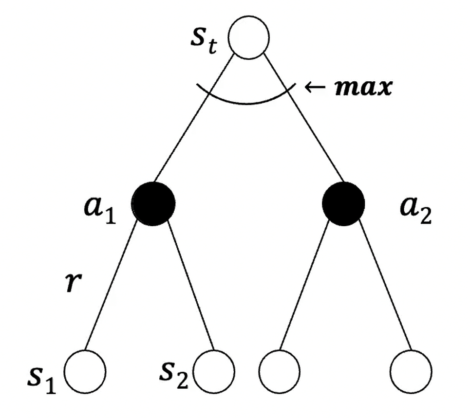
• White Node: Choose action with max value.
• Black Node: Average state values of all possible actions.
• Compute Optimal $Q(s,a)$ values for the current state by construction an expectimax tree.

$$Q(s,a)=\sum_{s'}P_\nu(s'|s,a) \left[R_\nu(s,a,s')+\gamma V(s')\right]$$ $$V(s)=\max_a Q(s,a)$$

• $P_\nu(s'|s,a)$: Transition probability.
• $R_\nu(s,a,s')$: Expected Reward
• $V(s')$: Value of the next state.

Limitations of Expectimax Tree

$$O((|\mathcal S|\times|\mathcal A|)^H)$$

• Scaling Exponentially with Depth: Tree size grows exponentially with depth $H$.
• $|\mathcal S|$: Number of possible states.
• $|\mathcal A|$: Number of possible actions.
• $H$: Depth of the tree.

Monte Carlo Search Tree, MCTS

• Given a model $\mu_v$
• Build a search tree rooted at the current state $s_t$, sample actions and next states.
• Iteratively Construct and update the tree by performing $K$ simulation episodes starting from the root node.
• Once search is finished, select the current action with maximum value in the search tree.

$a_t = \arg\max_{a \in A} Q(s_t, a)$

Aspect	MCTS	Expectimax Tree
Expansion	Construct partial search tree	Construct full search tree up to a given depth
Exploration	Select branches using UCB	Explore all possible branches
Evaluation	Estimate values using sampled returns	Calculate expected values using transition probabilities
Action Selection	Select actions based on estimated values	Select actions with maximum expected values
Computational Cost	Controlled by simulation budget	Exponential in search depth
Trade-off	More efficient, but approximate	More exhaustive, but computationally expensive

Tree Traversal

$$Q(s,a,i) = \underbrace{V_i}_{\text{Exploitation}} + \underbrace{c\sqrt{\frac{\ln n(s)}{n(s,a)}}}_{\text{Exploration}}$$

• Use Upper Confidence Bound (UCB) to select which branches to explore.
• $c$: Exploration coefficient.
• $n(s)$: Number of visits to state $s$.
• $n(s,a)$: Number of visits to state-action pair $(s,a)$.
• Exploration Bonus: Encourages selecting less-visited actions.
• UCB: Balances exploitation of high-value actions and exploration of less-visited actions.
  • In bandit problems, $c$ is a constant to balance exploration and exploitation.

Node expansion

• Add a new child node to the search tree for an unexplored action.

Rollout

• Perform a random simulation from the expanded node until termination or a depth limit.
• Calculate the total return from the simulation.

$$\begin{aligned} & \text{ROLLOUT}(S_i) \\ & \quad \text{Loop: } \\ & \quad \quad \text{if } S_i \text{ is a terminal } \\ & \quad \quad \quad \text{return } S_i \\ & \quad \quad \quad \text{else } \\ & \quad \quad \quad \quad A_i = \text{random available action } S_i \\ & \quad \quad \quad \quad S_i = \text{Simulate } (A_i, S_i) \\ \end{aligned}$$

Backpropagation

• Propagate the simulation return back through the selected path to the root.
• Update visit counts and estimated values of the visited nodes.

Advantages of MCTS

• Highly Selective Best-First Search
• Evaluates states dynamically, unlike DP.
• Use Samples to break curse of dimensionality.
• Works for "black box" model.
• Computationally efficient.

Reinforce Learning with Human Feedback, RLHF

Why Human Feedback?

• Some tasks do not have clear or automatically measurable rewards.
• Humans can provide:
  • Preferences: Choose between two outputs (A > B).
  • Rankings: Rank multiple outputs (1st, 2nd, 3rd).
  • Evaluations: Judge whether an answer is better or worse.
• Example: Evaluating which chatbot response is more polite.

Alignment Problem

• LLMs are pretrained to predict text, not necessarily to generate useful responses.
• Generated text may be harmful, biased, or factually incorrect.
• Traditional evaluation metrics (e.g., BLEU) do not directly capture human preferences.
• Human feedback helps align model behavior with human preferences for helpfulness, truthfulness, and safety.
• Example: A model may generate plausible but impractical coding advice.

Core Idea of RLHF

• Human Feedback: Use human evaluations and preferences to guide model training.
• Alignment: Align model behavior with human expectations and preferences.
• Optimization: Train models to maximize rewards reflecting human preferences rather than only next-token likelihood.
  • Goal of LLM's pretraining: $\max_\theta \sum_{t}\log P_\theta(x_t | x_{<t})$
    • Maximize the likelihood of the next token.
  • Goal of RLHF: $\max_\theta \mathbb{E}_{y \sim \pi_\theta(\cdot|x)} R(x, y)$
    • Maximize the expected reward of human-preferred responses.
• Application: Widely used in NLP and LLM alignment.

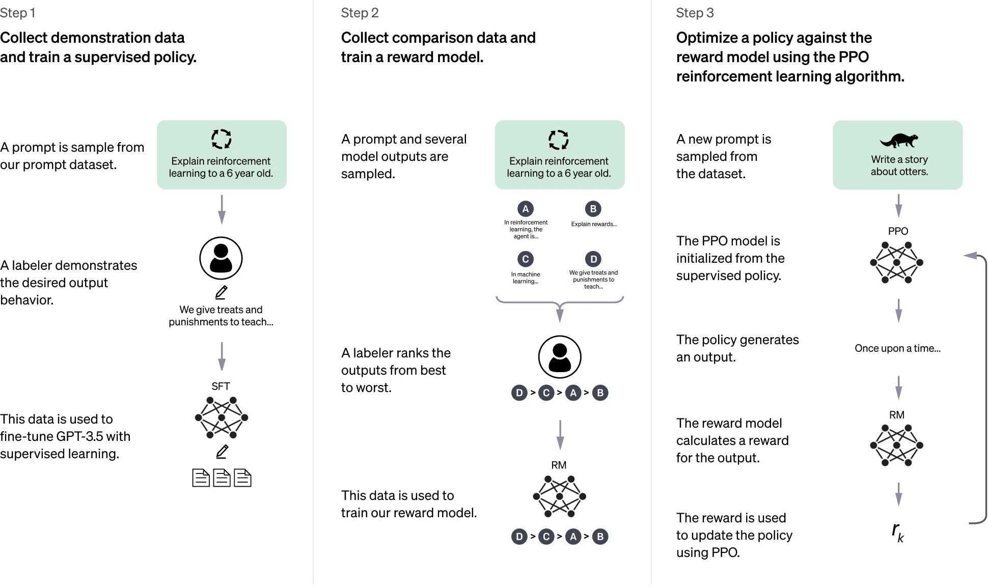
RLHF Training Pipeline

Pre-training → SFT → Reward Model Training → RL Optimization

1. Pre-training: Train a base model on a large text corpus using next-token prediction.
2. Supervised Fine-Tuning (SFT): Fine-tune the base model on high-quality instruction-response examples.
3. Reward Model Training: Train a reward model using human-labelled preferences to predict response quality.
4. Reinforcement Learning: Optimize the model's policy to maximize rewards predicted by the reward model.

Step 1. Pre-training

• Select a base model pretrained on a massive text corpus.
• Learns general knowledge and language patterns.
• Limitation: May produce biased, unsafe, or irrelevant responses.

Step 2. Supervised Fine-Tuning (SFT)

• Goal: Train the base model to follow instructions and generate reasonable responses.
• Collect high-quality demonstration data (instruction, input, output).
• Fine-tune the base model on the curated dataset.
• Limitation: Instruction-following does not guarantee alignment with human preferences.

Step 3. Reward Model Training

• Goal: Learn a reward function that reflects human preferences.
• Generate multiple responses for the same prompt.
• Humans compare or rank the responses.
• Train a reward model to assign scores based on human preferences.
• Example: A professional, polite response (B) is preferred over a blunt response (A): B > A.
• Outcome: Convert human judgments into numerical reward scores.

Step 4. RL with Human Feedback

• Goal: Optimize the LLM policy using the trained reward model.
• Algorithm: PPO (example).
• Generate responses using the current policy.
• Score responses using the reward model from Step 3.
• Update the policy to maximize reward.
• Use a KL penalty to limit deviation from the reference policy and reduce over-optimization.
  • KL Penalty: Penalizes large deviations between the updated policy and the reference policy.
  • Higher KL Penalty → More conservative policy updates.

$$D_{KL}(P\|Q)=\sum_x P(x)\log\frac{P(x)}{Q(x)}$$ $$\max_\theta\left[ \mathbb E[R(x,y)] -\beta D_{KL}(\pi_\theta\|\pi_{\mathrm{ref}}) \right]$$

Strategy	CNN	LLM
Feature Extraction	Freeze backbone, train classifier head	Freeze base model, train task-specific head
Partial Fine-Tuning	Freeze early layers, update selected layers	PEFT (e.g., LoRA): Freeze base weights, train small additional parameters
Full Fine-Tuning	Update all pretrained weights	Update all pretrained weights (not PEFT)

Chatgpt

Benefits of RLHF

• Alignment: Aligns model behavior with human values and preferences.
• Safety & Usefulness: Encourages safer, more useful responses with higher human acceptance.
• Ambiguous Goals: Handles tasks where rewards are difficult to define explicitly.

Challenges of RLHF

• Cost: Requires extensive human annotations, making training expensive.
• Human Bias: Biases in human feedback can be transferred to the reward model and policy.
• Over-optimization: Models may exploit the reward function rather than produce genuinely better responses (Reward Hacking).
• Scalability: Collecting and applying human feedback becomes difficult as models and tasks scale.

Applications of RLHF

• ChatGPT: Improvement in safety and helpfulness
• Claude: Constitutional AI for more nuanced alignment
• Gemini: Large-scale RLHF for multimodal capabilities
• Robotics: Learning task from human demonstrations
• Teaching robots via human feedback to cook
• Medical AI systems trained with doctor's feedback to align with human expert medical standards.