본문으로 건너뛰기

FDA +008

· 약 8분

Mearues of performance

Accuracy

A=TP+TNTP+TN+FP+FNA = \frac{TP + TN}{TP + TN + FP + FN}

  • the ratio of correct predictions to all predictions
  • it is the number of true positives and true negatives (the correct predictions) divided by the total number of predictions.

Error rate

E=FP+FNTP+TN+FP+FNE = \frac{FP + FN}{TP + TN + FP + FN}

  • the ratio of incorrect predictions to all predictions
  • It is equivalent to 1Accuracy1 – Accuracy.
  • It is the number of false positives and false negatives divided by the total number of predictions.

True positive rate, Recall, Sensitivity

TPR=TPP=TPTP+FNTPR = \frac{TP}{P} = \frac{TP}{TP + FN}

  • the proportion of actual positives for which the test result is positive.
  • it shows how sensitive the model is to detecting positive instances.
  • the ratio of true positives to all positives
  • the data points that were correctly predicted as positive divided by the number of true positives and false negatives.

False positive rate, Fall Out, False Alarm

FPR=FPN=FPFP+TNFPR = \frac{FP}{N} = \frac{FP}{FP + TN}

  • the proportion of actual negatives for which the test result is positive.
  • It is equivalent to 1Specificity1 – Specificity.
    • large values of specificity indicate small false negative rates.

The true negative rate, Specificity

SPC=TNR=TNN=TNFP+TNSPC = TNR = \frac{TN}{N} = \frac{TN}{FP + TN}

  • the proportion of actual negatives for which the test result is negative
  • It shows how well the model does at identifying actual negatives as negative.

The false negative rate, Miss Rate

FNR=FNTP+FNFNR = \frac{FN}{TP+FN}

  • the proportion of the actual positives for which the test result is negative.
  • It is equivalent to 1Sensitivity1 – Sensitivity.
    • large values of sensitivity indicate small false positive rates.
  • It is a common trick that often change classifiers to bias them towards making type 1 FP versus type 2 FN errors.
    • This can often change classifier to bias towards making FP errors rather than FN errors.
    • It depends on which are worse to make
    • They are biased if there are different numbers of items in each class

Precision, Positive Predictive Value

  • PPV, Positive Predictive Value
  • a measure of how accurate and precise the positive predictions are
  • It is the ratio of true positives to predicted positives.

Accuracy and Error rate

  • in practice, the previous measures don't always work well
    • they are biased, especially if there are different numbers of items in each class.
  • if the data is imbalanced, it's much better to use a true positive rate or true negative rate instead.

F1

F=2PrecisionRecallPrecision+RecallF = 2 * \frac{Precision * Recall}{Precision + Recall}

  • known as F-score or F-measure
  • a measure of the accuracy of the test
  • It is the harmonic mean of the recall and precision, where an F1 score reaches its best value at 1 (perfect precision and recall).
  • It allows the Recall and Precision to be assessed in the same calculation.
Predicted \ ActualPositiveNegativeTotal
Positive1105115
Negative106070
Total12065185
  • Accuracy=110+60185=0.91Accuracy = \frac{110 + 60}{185} = 0.91
  • ErrorRate=10+5185=0.08Error Rate = \frac{10 + 5}{185} = 0.08
  • TruePositiveRate(Sensitivity/Recall)=110115=0.95True Positive Rate (Sensitivity/Recall) = \frac{110}{115} = 0.95
  • FalsePositiveRate=1070=0.14False Positive Rate = \frac{10}{70} = 0.14
  • TrueNegativeRate(Specificty)=6070=0.85True Negative Rate (Specificty) = \frac{60}{70} = 0.85
  • FalseNegativeRate=5115=0.04False Negative Rate = \frac{5}{115} = 0.04
  • Precision=110120=0.91Precision = \frac{110}{120} = 0.91
  • F1=(20.910.95)/(0.91+0.95)=0.92F1 = (2 * 0.91 * 0.95) / (0.91 + 0.95) = 0.92

ROC curve

Receiver Operating Characteristic Curve

  • a graphical plot that explains how well a binary classifier system performs as the threshold at which it calls a data point as positive is varied.
  • ROC graphs were originally used in the communications area to look at false alarm rates.
  • The x-axis is the false positive
  • The y-axis is the true positive rate (sensitivity, recall)
  • ROC graphs contain all the information in the confusion matrix.
    • TPR(=TP/(TP+FN)), FPR(=FP/(FP+TN))
  • a visual tool to compare trade-offs between the ability of a classifier to correctly identify positive cases and the number of negative cases that are incorrectly identified.
  • an essential evaluation metric for checking the performance of a classification model.

AUC

Area Under the ROC Curve

  • AUC 0: the model predicts a negative class as a positive class and vice versa.
  • AUC 0.5: the model has no discriminative capacity to differentiate between negative class and positive class
    • diagonal line from (0,0) to (1,1)
  • AUC 0.7: 70% chance that the model will be able to differentiate between the positive and negative classes.
  • AUC 1: the model predicts all positive class as positive class and all negative class as negative class.
  • ROC is a probability curve and AUC represents the degree of separability
  • It shows how capable the model is of differentiating between the classes.

Training/testing split

  • train-test split procedure is used to estimate the performance of machine learning algorithms
  • should not be used
    • when the dataset is small
    • when the dataset is imbalanced
    • where additional configuration is required
    • train_test_split(..., stratify=y)
  • most common approach to validate model performance
    • traning data is 80%
    • testing data is 20%

k-fold cross-validation

  • helps select the model which will perform best on unseen data
  • overcoming the problem of overfitting and underfitting.
  • a parameter called k defines the number of portions that a given data sample will be split into.
  • k-fold cross-validation has less bias because it ensures that every single discovery from the main dataset has a chance to appear in both training and test sets.
Iteration of a 5-fold cross-validation

# X = Test set
# T = Train set
1st fold : XXXX TTTTTTTTTTTTT
2nd fold : TTTT XXXX TTTTTTTT
3rd fold : TTTTTT XXXX TTTTTT
4th fold : TTTTTTTT XXXX TTTT
5th fold : TTTTTTTTTTTTT XXXX
k = 3
dataset = [1, 2, 3, 4, 5, 6]

fold1 = [5, 2]
fold2 = [1, 3]
fold3 = [4, 6]
  • Model1 will be trained on fold1 and fold2, and tested on fold3
  • Model2 will be trained on fold2 and fold3, and tested on fold1
  • Model3 will be trained on fold1 and fold3, and tested on fold2
  • we can take the accuracy as the average of all rounds to get the final accuracy.

Bias-variance decomposition

a formal method for understanding the prediction error of a model.

  • the average of the distance between the target and model predictions.
  • simple model: High bias, Low variance → Underfitting
    • not complex, high error component
  • complex model: Low bias, High variance → Overfitting
    • quite sensitive to the specific training set

Bias

the average of the distance between the target and model predictions.

  • how well the model can do for any training set.
  • the difference between the expected value and the parameter that we want to estimate
  • Bias=E[θ^]θ\text{Bias} = E[\hat{\theta}] - \theta
    • If the bias is exactly zero, the estimator is unbiased
    • If the bias is greater than zero, the estimator is positively biased
    • If the bias is less than zero, the estimator is negatively biased

Variance

the deviation between the average prediction value and the predicted value.

  • Classifier error is also affected by variability in the training data because different training sets lead to different decision boundaries.
  • High variance: it produces different results for different training sets.
    • sensitive to the particular training set.
    • models with less parameters tend to have lower variance.
  • Var(θ^)=E[(θ^E[θ^])2]Var(\hat{\theta}) = E[(\hat{\theta} - E[\hat{\theta}])^2]

Noise

changes in the target value

  • objects with the same attribute values leading to different class labels.
  • these errors are unavoidable even when you know the correct decision boundary.

Evaluating

Underfitting

the model did not capture enough patterns in the data

  • The model provides poor performance on both the training and the test set.
  • Reasons:
    • The training model is not trained as tightly as possible.
    • The model is not able to learn more.
      • model is not suitable for the task.
  • Avoid underfitting by:
    • using more training data
    • choosing / training a more complex model
    • increase the number of parameters in the model, the type or complexity of the model, or the traninig time till a cost function is minimized.

Overfitting

the model captures noise and patterns which do not generalize well to new data.

  • The model has extremely good performance on the training set, but poor performance on the test set.
  • Reasons:
    • the training data is not a perfect standard
  • Avoid overfitting by:
    • regularization
    • pruning (parameters, strucutres of classifiers)
    • reducing the descriptive length (minimize the sum of the model's complexity and the dscription of the traning data)
    • optimization (use a separate subset for validating the model)
    • expansion (use or generate more training data)
      • adding synthetic samples to the dataset.

K-NN

k-Nearest Neighbors

  • a non-parametric technique
    • not involving any assumptions as to the form or parameters of a frequency distribution
  • supervised learning classifier
    • uses proximity to make classifications or predictions about the grouping of an individual data point
    • defining new cases based on similarity measures (e.g., distance functions).
    • Euclidean: d(x,y)=(xiyi)2d(x, y) = \sqrt{\sum_{} (x_i - y_i)^2}
    • Minkowski: d(x,y)=(xiyip)1/pd(x, y) = (\sum_{} |x_i - y_i|^p)^{1/p}
    • Hamming: d(x,y)=xiyid(x, y) = \sum_{} |x_i - y_i|
  • In weighted k-NN, weigh the votes according to distance
    • wi=1d2w_i = \frac{1}{d^2}
  • If k is too small, it may be sensitive to noise points
  • If k is too large, its neighbourhood may include points from other classes
  • Choose an odd value for k, to eliminate ties

Industrial Applications of KNN

  • Retail business data analysis: Identify customer patterns and generate business value.
  • Security and operational management: Simplify daily operations such as theft prevention.
  • Credit card usage monitoring: Detect unusual patterns to identify fraudulent transactions.
  • Transaction scrutiny software: Spot unfamiliar patterns and flag suspicious activity.
  • Point-of-sale (POS) data analysis: Analyse register data for operational insights.

IAI +007

· 약 8분

Computer vision

  • a field of artificial intelligence enabling computers and systems to derive meaningful information from digital images, videos and other visual inputs.
  • vision is a perceptual channel that accepts a stimulus and reports soome representation of the world
  • computer vision enables intelligent agents to see, observe and understand of environment

Core problems of CV

  • reconstruction: an agent builds a mode lfo the world from an image or a set of images
  • recognition: an agent draws distinctions amont the objects it encounters based on visual and other information.
    • image classification
    • object detection
    • image segmentation

Classic approaches to object recognition problems

  • feature-based object recognition approach
    • works well for faces looking directly at the camera.
  • pattern-element-based object recognition approach
    • a useful abstraction is to assume that some objects are made up of local patterns which tend to move around with respect to one another.
    • we can model objects with pattern elements.

Modern approaches to object recognition problems

  • deep learning networks
    • to recognition problems enables that features can be automatically learned and extracted from raw image data compares with the manual feature extraction in the classic approaches.
    • AlexNet, VGGNet, GoogleNet, ResNet, DenseNet, EfficientNet, RegNet...
  • basic models and derived models
    • YOLO, SSD, RetinaNet, R-CNN...

Evaluation metrics for image classification

MetricDefinitionUse case
Accuracythe percentage of correcly predicted labels out of all predictions madecommonly used in balanced datasets but can be mis leading in imbalanced classes
Precisinothe ratio of correctly predicted positive observations to the total predicted positives.useful when the cost of false positives is high (e.g., spam detection)
Recall (Sensitivity or True Positive Rate)the ratio of correctly predictted observations to all the actual positivesimportant when the cost of false negatives s high (e.g., disease detection)
F1 Scorethe harmonic mean of Precision and Recallused when you need to balance precision and recall, especially in imbalanced datasets
Specificity (True Negative Rate)the ratio of correctly predicted negative observations to all the actual negatives.important when false positives should be minimized (e.g. medical tests for diseases)
Confusion Matrixa table used to describe the performance of a classification model by showing the true positive, false positive, true negative, and false negative countsprovides a comprehensive understanding of a models' performance across all classes
ROC Curve (Receiver Operation Characteristic)a graphical representation of the classifier's performance across all thresholds, plotting the true positive rate (recall) against the false positive rate (1 - specificity)used to evaludate binary classirifres and compare models
AUC (Area Under the Curve)the area under the ROC curve, providing a single number summary of the models' ability to discriminate between positive and negative classesuseful for evaluating binary classification models, particularly when dealing with imbalanced datasets.

Confusion Matrix

Actual class ➡️
Predicted class ⬇️
PositiveNegativeMetric
PositiveTP: True PositiveFP: False PositivePrecision: TPTP+FP\frac{TP}{TP + FP}
NegativeFN: False NegativeTN: True NegativeNegative Predictive Value: TNTN+FN\frac{TN}{TN + FN}
MetricRecall or Sensitivity: TPTP+FN\frac{TP}{TP + FN}Specificity: TNTN+FP\frac{TN}{TN + FP}Accuracy: TP+TNTP+TN+FP+FN\frac{TP + TN}{TP + TN + FP + FN}

ROC Curve

  1. Sort predicted probabilities
  2. Try multiple thresholds
  3. For each threshold, compute predicted labels
  4. Compute TPR and FPR
  5. Plot ROC curve (FPR vs TPR) i. TPR=TPTP+FNTPR = \frac{TP}{TP + FN} ii. FPR=FPFP+TNFPR = \frac{FP}{FP + TN}
  6. Compute AUC as area under ROC curve
from sklearn.metrics import roc_curve, roc_auc_score
fpr, tpr, thresholds = roc_curve(y_true, y_scores)
auc = roc_auc_score(y_true, y_scores)

Evaluation metric for object detection

MetricDefinitionUse case
Intersection over Union (IoU)measures how much the predicted bounding box overlaps with the ground truth.IoU=Area of OverlapArea of UnionIoU = \frac{\text{Area of Overlap}}{\text{Area of Union}}
Precisionthe ratio of correctly predicted postive observations to the total predicted positivesPrecision=TPTP+FPPrecision = \frac{TP}{TP + FP}
Recallthe ratio of correctly predicted observations to all the actual positivesRecall=TPTP+FNRecall = \frac{TP}{TP + FN}
F1 Scorethe harmonic mean of Precision and RecallF1=2×PrecisionRecallPrecision+RecallF1 = 2 \times \frac{Precision \cdot Recall}{Precision + Recall}
Average Precision (AP)Precision-Recall Curve: Precision vs Recall at different thresholds
AP: Area under the Precision-Recall curve (per class)
AP=01P(r)drAP = \int_{0}^{1} P(r) \, dr
Mean Average Precision (mAP)mean of AP across all classesprovides a comprehensive understanding of a models' performance across all classes
AP@[.50:.95]COCO benchmarkAverages AP at IoU threshold from 0.5 to 0.95 in steps of 0.05
  • AP is computed by summing trapezoid areas under the Precision-Recall curve.

Convolutional Neural Network (CNN)

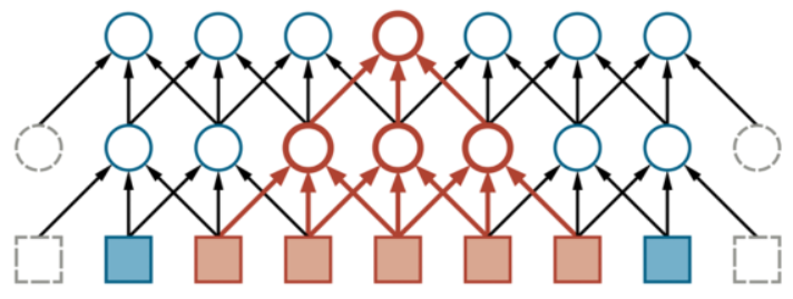
  • contains spatially local connectinos at lest in the early layers
  • has patterns of weights that are replicated across the units in each layer.
  • use a kernel to detect patterns of weights that is replicated across multiple local regions in an image
  • use convolution that applies the kernel to the pixels of the image
Input

[Conv → ReLU][Pooling]

[Conv → ReLU][Pooling]

Flatten (2D → 1D 벡터)

Fully Connected Layer

Output Layer (Softmax/Sigmoid)

zi=j=1lkjxj+(i1)sz_i = \sum_{j=1}^{l} k_j \cdot x_{j + (i-1)s}

  • ziz_i: the ii-th output element (convolution result)
  • jj: index inside the kernel (from 1 to ll)
  • ll: kernel size (number of elements in the kernel)
  • kjk_j: the jj-th kernel weight (filter element)
  • xx: input sequence (the original data)
  • xj+(i1)sx_{j+(i-1)s}: the input element aligned with kernel position jj when shifted by stride
  • ss: stride (step size of the kernel movement)
  • (i1)s(i-1)s: total shift in the input for the ii-th convolution

Receptive Field

  • the receptive field of a neuron is the portion of the sensory input that can affect aht neuron's activation.
  • In CNNs, the receptive field of a unit in the first hidden layer is small.
  • just the size of the kernel, e.g., 3x3 or 5x5.
  • In the deeper layers of the network, it can be much larger.

1D CNN

RL=RL1+(kL1)i=1L1siR_{L} = R_{L-1} + (k_{L} - 1) \cdot \prod_{i=1}^{L-1} s_i

  • RLR_L: receptive field size at the LthL-th layer
  • kLk_L: kernel size at the LthL-th layer
  • sis_i: stride at the ithi-th layer
LayerKernel kStride sCalculationResult RF
Conv1311 + (3-1)*13
Pool1223 + (2-1)*14
Conv2314 + (3-1)*28

Pooling

  • works like a convolutional layer, with a kernel size ll and stride ss, but the operation is applied is fixed rather than learned.
  • no activation fucntion is associated with the pooling layer.
  • common forms of pooling
    • average pooling
    • max pooling: saying a feature exists somewhere in the unit's receptive field.

Dropout

  • a way to reduce the test-set error of a network to increase its ability of generalization.
  • makes a etwork herder to fit the traninig set.
  • the network is created by deactivating a randomly chosen subset of the units (dropout rate).
  • cannot explain why it works but the results is better

Batch Normalization

  • modern neural networks are almost always trained with some variant of stochastic gradient descent (SGD).
  • Batch normlization rescales the values generated at the internal layers of the network from the examples within each minibatch.
    • it standardizes the input to a layer for each mini-batch.
  • standardizes the mean and variance of the values.
  • maeks it much simpler to train a deep network.

Tranining in a CNN

Crossentropy(y,y^)=iyilog(y^i)Cross-entropy(y, \hat{y}) = -\sum_{i} y_i \log(\hat{y}_i)

  • Forward pass
  • Backward pass
  • Parameter update

Variants of CNNs

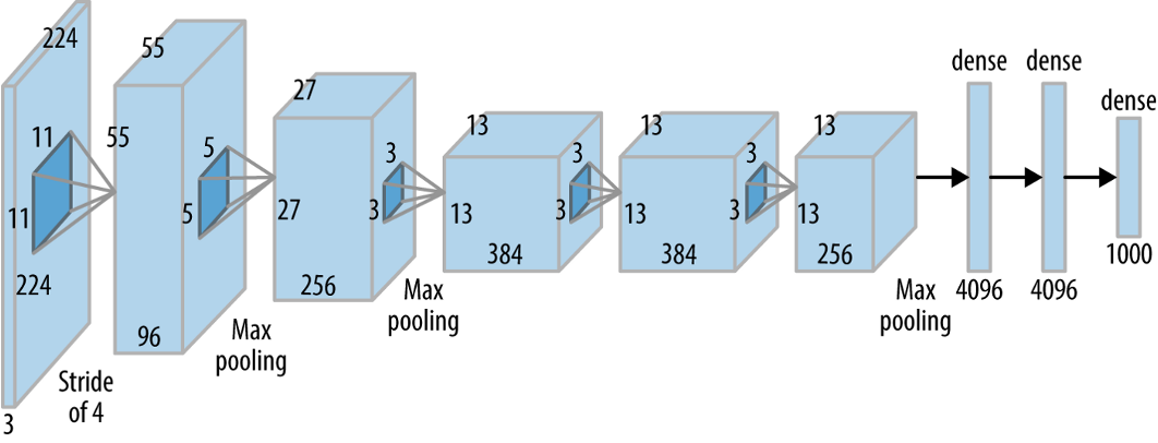
AlexNet

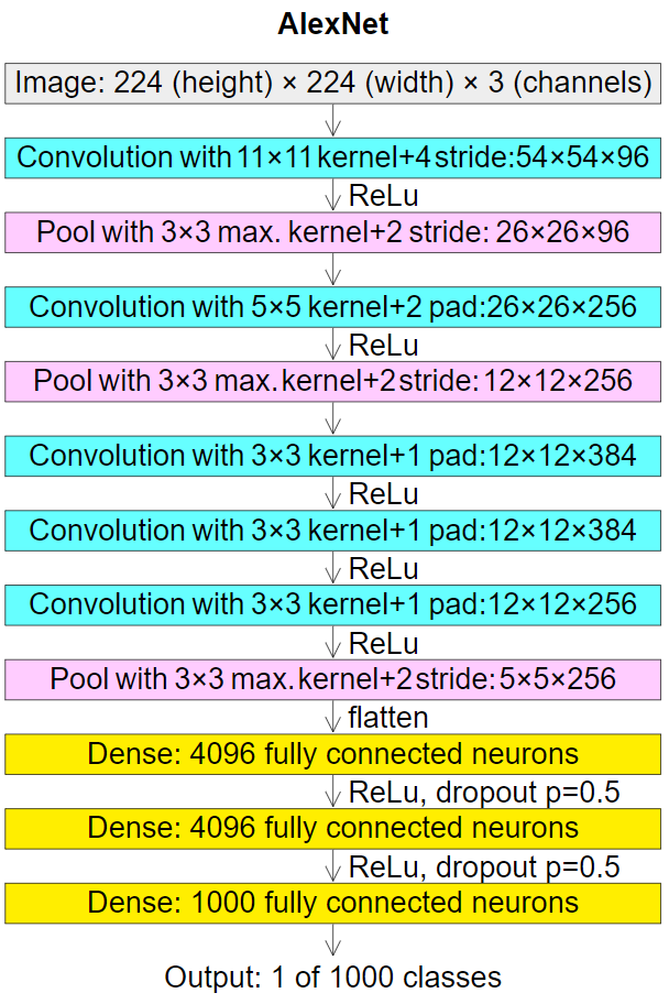
AlexNet

AlexNet Layers

ResNet

  • stands for a residual neural network.
  • was designed to enable hundreds or thousands of convolutional layers.
  • Residual neural networks do this by utilizing skip connections, or shortcurts to jump over some layers.
  • was an innovative solution to the "vanishing gradient" problem.
x ────────────────► (+) ──► y
│ ▲
▼ │
[Conv → ReLU → Conv] = F(x)

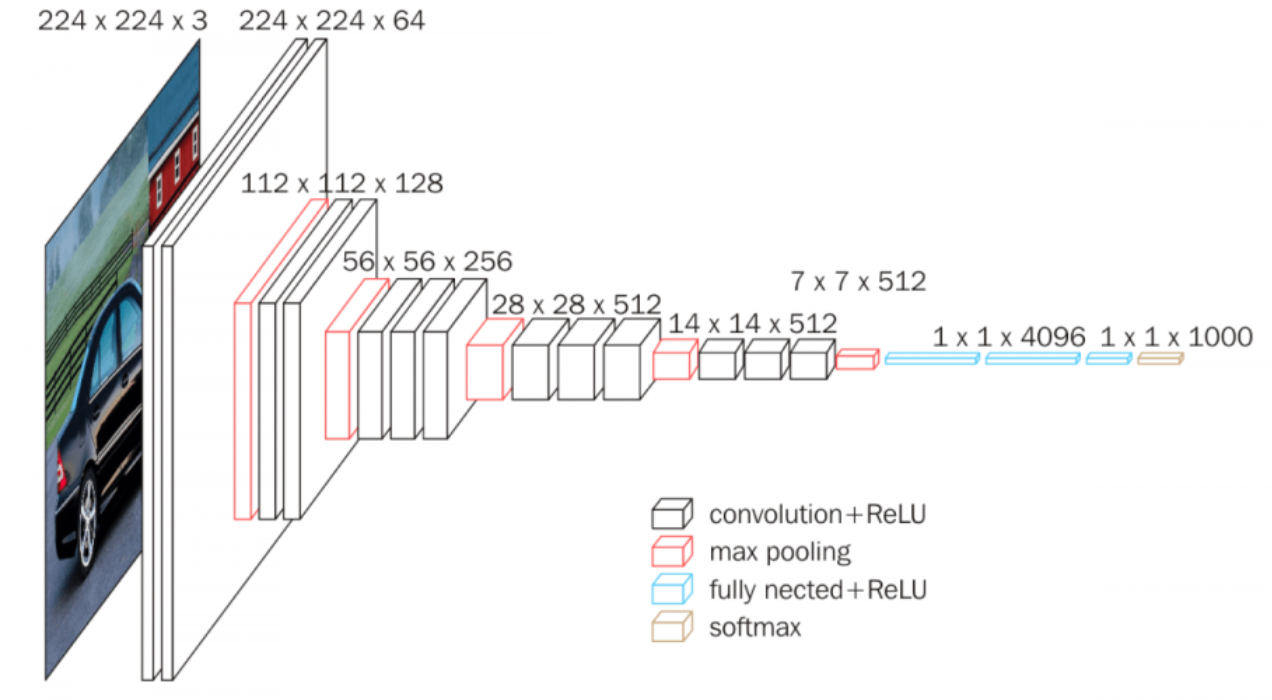
VGGNet

  • increases the depth of the network through adding more convolutional layers by using small convolution filters (3x3) while other parameters are fixed.

VGGNet

Derived model for object detection

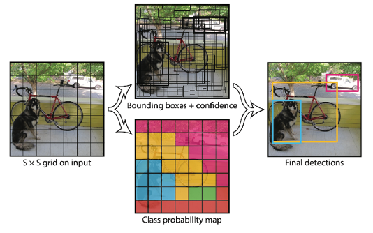
YOLO

  1. Split an images to S times S blocks.
  2. Apply object classification to each block and get confidence score of different objecxt for each block.
  3. Based on the class probability map to locate objects.

YOLO

Calculation AP and mAP

  1. Gather Detection results
  2. Match Predictions to Ground Truth
  3. Compute Precision and Recall to generate a set of (recall, precision) points
  4. Build the Precision-Recall (PR) Curve (presioin decreases as recall increases)
  5. Smooth the Precision-Recall Curve
  6. Calculate AP
  7. Extend to mAP

FSD +008

· 약 5분

OOP Principles

Encapsulation

  • bundles data attributes (fields) with methods that use the data in a single unit called "Object"
  • hides sensitive data attributes by declaring the fields private.
  • fields can be declared protected in the parent class, allowing access from the child class.
  • exposes the data attributes values only through public getters/setters to allow access or modification of the field values.

Intheritance

class A:
pass

class B(A):
pass

class C(A):
pass
  • Superclass defines common method signatures (with/without implementation) and fields.
  • Subclasses provide the implementations for (or override) these method signatures
  • private attributes cannot be directly accessed from the child classes.
  • to refer to superclass properties (fields, methods) or constructor, use the keyword super()

Polymorphism

  • means many forms.
  • permits an object to have multiple types.
  • allows object of different types but with a common parent to be stored in the same collection.
  • enables inherited methods from the parent to perform different tasks when called by subclasses.

Abstraction

  • the process of hiding the implementation details and exposing only the necessary behavior to the user.
  • abstract class must at least contain one abstract method.
  • abstract class ccan have concrete methods.
  • abtract methods are only prototypes in the parent class, the actual implementation is provided by the subclasses that inherit the abstract class.
  • rules
    • if a class contains at least on abstract methods, it should be declared abstract.
    • if another class inherits an abstract class, it must implement all the abstract methods of that class.
from abc import ABC, abstractmethod

class Person(ABC):
def __init__(self, name):
self.name = name

@abstractmethod
def show(self):
pass

def show_name(self):
print(f"Name: {self.name}")

class Student(Person):
def __init__(self, name, id):
self.id = id
super().__init__(name)

def show(self):
super().show_name()
print(f"ID: {self.id}")
  • interfaces are complete abstract classes declared with the interface keyword.
  • only contain prototype (abstract) methods with empty body code.
  • cannot be instantiated nor inherited as they do not have constructors.
  • a class can implement multiple interfaces.
  • a class implementinig an interface must provide an implementation for all its abstract methods.
  • add an access layer to further hide the methods impelmentation.
  • act as a middleware inside the program, allowing human, machines, and other software to interact with the program's functionalities without knowing the implementation details.
# interface A is a fully abstract class
# interface A must inherit ABC
# class B(A) must implement all abstract methods of A
# interface A methods have the @abstractmethod decorator with pass as body-code
from abc import ABC, abstractmethod

class Person(ABC):
@abstractmethod
def show_info(self):
pass

class Student(Person):
def __init__(self, name, id):
self.name = name
self.id = id

def show_info(self):
print(f"Name: {self.name}, ID: {self.id}")

OOP Design Rules

  • How to split the code into seperate classes and preserve encapsulation
  • How to organizae the code into methods to hide the implementation details and expose the behavior
  • How the objects interact at runtime
  • How to name the class entities

5 Design Rules

  • Encapsulation
    • hide fields behind methdos
    • requires fields to be private while allowing methods to be public
    • requires a methods related to a field (such as access, modify, use) be defind in the same class.
  • Push code to the right
    • requires the code/methods used by objects of a class be written in the same class.
    • ensures methods are written for reusability and placed in the correct class so they can make use of the class's fields.
    • determines which class is responsible for defining the methods needed to achieve the program's goals.
  • Spread plans across classes
    • involves planning the distribution of code across multiple classes from the start.
    • focuses on distributing responsibilities logically among different classes, so that each class has a clear and focused role.
    • by convention, this rule requires using the same method name (for the same goal) across all classes.
  • Hide by default
    • hiding implementation details within a class and exposing only the necessary functionality to the outside.
    • helps in achieving encapsulation and abstraction.
    • promotes better design and maintainability.
  • Follow naming conventions
    • use nouns to name fiels.
    • use nouns to name functions.
    • use verbs to name procedures.
    • if an entitiy is compsed of two or more words.
      • use camelCase/snake_case for fields and methods.
      • use PascalCase for class names.
  • consolidates the action-trieggers of a program into a single method.
  • common design choice in applications with user interaction.
  • the menu methods is executed in the program's main method.
    • offers users interactive CLI command choices.
  • menu() requires a read-function in a while loop, allowing the menu() tor repeatedly read inpus from STDIN.
<condition> = read_choice()

loop (<condition>):
check (<condition>):
case 1: do task <action_1()>
case 2: do task <action_2()>
...
case n: do task <action_n()>
default: <alternative-action>
menu(self):
choice = input("Enter choice: (d/w/b/h/x): ").lower()
while choice != "x":
match choice:
case "d":
self.deposit()
case "w":
self.withdraw()
case "b":
self.show_balance()
case "h":
self.show_history()
case "x":
self.exit()
case _:
self.show_invalid_choice_message()

choice = input("Enter choice: (d/w/b/h/x): ").lower()

FDA +007

· 약 7분

Classification and Prediction

Classification

classifies data based on the training set and the class labels and uses it in classifying new data

  • Model construction (learning)
  • Model evaluation (accuracy)
  • Model use (classification)

Prediction

predicts categorical class labels based on unseen data

  • models continuous-valued functions

Classfication Methods

  • Decision tree induction
  • Bayesian classification
  • Nearest neighbour classification, case-based reasoning
  • Neural networks
  • Support Vector Machines
  • Ensemble methods

Issues around classification and prediction

  • Predictive accuracy
  • Speed and scalability
  • Robustness
  • Interpretability
  • 'Goodness' of classifier

Classification process

Decision Tree

  • Builds trees to describe data
  • Easy to translate into rules
  • Robust to niosy data
  • able to build disjunctive expressions
  • Inductive bias prefers small trees over larger.

Decision Tree Methodologies

  • Itertative Dichotomiser 3 (ID3)
  • C4.5
  • Classification And Regression Trees (CART)
  • Chi-square Automatic Interaction Detection (CHAID)
  • Multivariate Adaptive Regression Splines (MARS)

Decision Tree Forms

  • Balanced
    • each branch has the same depth from the root to leaves.
    • all nodes have the same number of splits
  • Deep
    • some nodes have different levels, wherein some of them are split into more branches.
  • Bushy
    • split into multi-way from the root
    • undesirable because the split may lead to small numbers of instance in each leaf node.

Entropy and Information Gain

Entropy

measures the amount of disorder / (im)purity in a collection of things. i.e. the unpredictability of the data.

Entropy(S)=p+log2(p+)plog2(p)Entropy(S) = -p_{+} log_2(p_{+}) - p_{-} log_2(p_{-})

  • Constructing a decision tree is all about finding an attribute that returns the highest information gain and the smallest entropy.
  • SS stands for total number of samples
  • P+P_{+} denotes the likelihood of a yes (positive) answer.
  • PP_{-} denotes the likelihood of a no (negative) outcome.

E(S)=i=1cpilog2(pi)E(S) = \sum_{i=1}^{c} -p_i log_2(p_i)

Information Gain

measures how well a given attribute separates the training examples according to the target classification.

  • The larger the information gain is, the stronger the feature will be.

Gain(S,A)=Entropy(S)vValues(A)SvSEntropy(Sv)Gain(S,A) = Entropy(S) - \sum_{v \in Values(A)} \frac{|S_v|}{|S|} Entropy(S_v)

  • SS = set of training examples
  • AA = the particular attribute to be tested
  • Values(A)Values(A) = the set of values for the attribute A
  • SvS_v = subset of SS with attribute AA having value vvs

Iterative Dichotomiser 3

  • constructs trees in a top-down manner.
  • check each instance attribute with a statistical test to see how well it alone classifies (splits) the training examples.
  • this becomes the root node.
  • descendent is created for each possible value of the attribute and training examples split to the appropriate descendent.
  • repeat the procedure for each descendent.
  • the algorithm is going to issue recursion on each of the partitions.
  • the output of this algorithm is the creation of a Model.
function id3 (examples, target, attrs):
create root node for tree

if examples all +ve, return root with label=+
if examples all -ve, return root with label=-
if attrs is empty
return root w/ label=most common value of target in examples else
else
A ← attribute from attrs that best splits examples
root ← A for each possible value, vi , in A
add a new branch below root corresp. to the test A = vi
examples_v ← the subset of examples with A = vi

if examples_vi is empty
add a leaf node below branch w/ label = most common value of target from examples
else below the branch add the subtree given by
id3(examples_vi , target, attrs - {A})

return root
  • ID3 can be seen as a search through a space of hypotheses for one that matches the training data.
  • It's a greedy search
  • Hypothesis space = all the possible trees
  • Simple to complex, hill climbing search
  • Complete search = decision tree can represent all possible hypotheses
  • Maintains only one current hypothesis
    • cannot find alternative decision trees
  • No backtracking, maybe stuck in local optima
  • Uses all training data at each step
    • less sensitive to errors in individual examples

Inductive Bias

  • Shorter trees preferred
  • High information gain near the root
  • cos' simple to complex search

Issues with decision trees

Overfitting training data

  • occurs when a tree gives higher accuracy on the training data than another tree, but lower accuracy on the unseen data.
  • because the training data is noisy or not representative of the unseen data.
  • can measure how well the tree generalizes by checking error on test data.

Dividing the data

  • Training set
    • used to build the initial model
    • may need to enrich the data to get enough of the special cases
  • Cross validation set
    • used to adjust the initial model
    • used to work out the correct values of parameters in model
    • models can be tweaked to be less dependent on idiosyncrasies in the training data to be a more general model
    • idea is to prevent over-training (i.e. finding patterns where none exist)
  • Test set
    • used to evaluate the model performance

Avoiding Overfitting

  • stop growing the tree once the test error decreases
  • grow the tree as normal (i.e. wit hoverfitting) then post-prune it.
  • use a separate set of data apart from training to test when to prune nodes (training & cross-validation set)
  • use all data to train, but apply a statistical test whether to expand/prune a node.
  • use an explicit complexity measure (e.g. Minimum Description Length, MDL) to trade off accuracy vs complexity.

Reduced-Error pruning

  • build tree
  • consider each node in tree for pruning
  • pruning
    • remove subtree
    • make into a leaf
    • assign label as most common class in associated training examples.
  • if pruned tree has as good error on the cross validation set as the unpruned tree, do the prune.
  • keep pruning until the error on cross validation set increases.

Cross validation set

  • the main difficulty comes when you don't have much data and need it all for training.
  • k-fold cross-validation or leave-one-out training can help.

Rule Post-Pruning

  • converts the decision tree to rules
  • removes preconditions that do not worsen the accuracy (on the cross validation set or with a statistical test)
  • sorts the rules by estimated accuracy and uses this order when classifying new data

Continuous Valued Variables

  • use real valued attributes for tests at nodes.
  • Dynamically define new discrete attributes that partition the continuous attribute.
  • discrete: A<v=trueA < v = true and A>=v=falseA >= v = false
  • the boundary poins can be estimated from the training data.

The confusion matrix

  • a basic method of evaluation of classifiers
  • The columns have numbers associated with the actual number of positive data points in the test set and the actual number of negative data points in the test set
Predicted PositivePredicted Negative
Actual PositiveTrue Positive (TP)False Negative (FN)
Actual NegativeFalse Positive (FP)True Negative (TN)
  • TP: the number of correct prediction of positive samples.
    • the number of data points in the test set that were positive and the classifier correctly assigned them to the positive group
  • TN: the number of correct prediction of negative samples
    • the number of data points in our test set that was actually negative and predicted as negative by the classifiers
  • FP: the number of incorrect predictions of positive samples
    • the value of data points in our test set that was actually negative but were predicted by the classifier as positives.
    • These ones are obvious errors, which is called a type 1 error.
    • type I error
  • FN: the number of incorrect prediction of negative samples.
    • the number of data points in our test set that was actually positive but were predicted by the classifier as negative
    • usually called the type 2 error, and when we are trying to build a classification.
    • might have a trade-off between the number of the type 1 error or the type 2 error.
    • type II error

Vocabulary for AI 008

· 약 3분

Vocabulary & Expressions

Term/ExpressionDefinitionSimpler ParaphraseMeaning
invariancethe quality of remaining unchanged when something else changesunchangingness불변성
disjunctiona logical operation that outputs true whenever at least one of its inputs is trueor operation논리합, OR
convergencethe process of coming together to a common pointcoming together수렴
impracticallynot in a practical or realistic mannernot practical비현실적으로
receptora cell or group of cells that receives stimuli and transmits them to sensory nervessensor수용체, 감각기
sensationthe process of sensing our environment through touch, taste, sight, sound, and smellfeeling감각
diffusespread out over a large area; not concentratedspread out확산되다
albedothe proportion of the incident light or radiation that is reflected by a surfacereflectivity반사율
color constancythe feature of the human color perception system which ensures that the perceived color of objects remains relatively constant under varying illumination conditionsconsistent color perception색채 항등성
occlusionthe blocking of light or other radiation by an objectblockage폐색, 차폐
deformationthe action or process of changing in shape or distorting, especially through the application of pressuredistortion변형
foreshorteningthe visual effect or optical illusion that causes an object or distance to appear shorter than it actually is because it is angled toward the viewerperspective shortening단축, 단축법
courtesyprovided at no costfree of charge무료 제공
apprenticeship learninga type of learning where an agent learns to perform tasks by observing and imitating a more experienced agentlearning by imitation도제 학습
consolidatemake (something) physically stronger or more solidstrengthen강화하다
aquamarinea light bluish-green colorlight blue-green아쿠아마린
fulvousa dull yellowish-brown colordull yellow-brown황갈색의
verbatimin exactly the same words as were used originallyword for word말 그대로, 축어적으로
lexiconthe vocabulary of a person, language, or branch of knowledgevocabulary어휘집
adherentsomeone who supports a particular party, person, or set of ideassupporter지지자
syntactic consitituenta word or a group of words that function as a single unit within a hierarchical structuresentence unit구문 성분
pragmaticsthe branch of linguistics dealing with language in use and the contexts in which it is usedlanguage use화용론
casea grammatical category that marks the relationship between a noun and other words in a sentencegrammatical role
persona grammatical category that distinguishes between different participants in a conversation (e.g., first person, second person, third person)participant distinction인칭
numbera grammatical category that expresses count distinctions (e.g., singular, plural)count distinction
headthe main word in a phrase that determines its syntactic typemain word중심어
separabilitythe quality of being able to be separated or divideddivisibility분리 가능성
intrinsicbelonging naturally; essentialinherent본질적인
기법아이디어비유
Laplace (Add-One)모든 경우의 수에 +1을 더해줌. 안 본 것도 최소한의 기회를 줌.시험 점수를 0점 맞아도 최소 1점은 줘
Backoffn-gram이 없으면 더 짧은 n-gram으로 내려가서 확률을 씀.3단어 조합 못 봤네? → 그럼 2단어 조합으로 보자 → 그것도 없으면 1단어라도 보자.
Linear Interpolation여러 레벨(n=1,2,3)을 동시에 섞어서 확률 계산.국어, 영어, 수학 점수를 일정 비율(λ)로 합쳐서 성적 보는 것.
Witten-Bell / Kneser-Ney더 정교하게 확률 질량을 재분배. (현업에서 성능 좋음)선생님이 본 적 없는 문제지만 유사 문제를 잘 풀었으니 점수 좀 더 주자 하는 것.
Stupid Backoff대충 큰 코퍼스를 모아서, 그냥 단순 backoff만 사용. (빅데이터 시대 구글에서 씀)데이터가 워낙 많으니까, 그냥 단순한 방법도 잘 먹힌다.

IAI +006

· 약 8분

Markov process or Markov chain

the state sequence satisfies the Markov assumption

  • The current state depends on only a finite fixed number of previous states.
  • P(XtX0:t1)=P(XtXt1)P(X_t | X_{0:t-1}) = P(X_t | X_{t-1})

Decision Theory

  • Choosing actions based on the desirability of their immediate outcomes.
  • The outcome of taking action aa in state s0s_0 is deterministic then Result(s0,a)Result(s_0, a).
  • If the outcome is non-deterministic (stochastic), fully observable, the agent knows the current state s0s_0.
    • It is represented as a random variable whose values are the possible outcome states.
    • The transition model specifies the probabilities of possbile outcome states.
    • P(s,a,s)P(s, a, s')

MEU, Maximum Expected Utility

A rational agent should choose the action that maximizes its expcted utility.

  • The MEU principle could be seen as defining all of AI.
  • action=argmaxa(EU(ae))action = argmax_a(EU(a|e))
    • among this set of actions, give the highest expected utility.
  • EU(ae)=s(P(Result(a)=sa,e)U(s))EU(a|e) = \sum_{s'} (P(Result(a) = s' | a, e) * U(s'))

Sequential decision problem

type of problem or scenario where a decision-maker must make a series of choices or decisions over time in order to achieve a desired outcome.

  • a sequential decision-making problem or sequential decision-making task

MDP, Markov Decision Process

a sequential decision problem for a fully observable, stochastic environment environment with a Markovian transition model and additive rewards.

  • a formal framework for modeling sequential decision problems.
  • including states, actions, transition probabilities, and rewards
  • used in reinforcement learning and operations research.
ComponentDescription
Environmentfully observable, Stochastic
Statesa set of states (with an initial state S₀)
Transition modelMarkovian
Rewardadditive
AgentMake decisions at time step for actions
Interacts with environment through percepts and actions
  • A set of states: an initial state S0S_0, possible terminal state(s)
  • A set of actions in each state: ACTIONS(s)ACTIONS(s)
  • A stochastic Markov transition model: P(ss,a)P(s' | s, a)
  • A reward function: R(s)R(s) or R(s,a,s)R(s, a, s')
  • In MDP, Additive Reward is defined as a function that assigns a numerical value to each state-action pair or state-transition pair.
    • represents the immediate benefit or cost associated with taking a specific action in a particular state.
  • The solution must specify what the agent should do for any state that the agent might reach.
  • Policy: π(s)π(s), an action for each state
    • A solution to an MDP.
    • π(s)\pi(s) is the action recommended by the policy π\pi for state ss
  • Q state: Q(s,a)Q(s, a), the expected utility of doing action aa in state ss

RL, Reinforcement Learning

  • an agent interacts with an environment
  • takes actions to maximize a cumulative reward signal over time.
  • learns a policy that balances exploration and exploitation
    • exploration: trying new actions.
    • exploitation: choosing known good actions.

Sample MDP

Environment

  • The agent lives in a 4x3 fully observable stochastic environment
  • Walls block the agent's path; Begin in the start state, the agent must choose an action at each time step
  • Actions available to the agent in each state: Up, Down, Left, or Right
  • The interaction with the environment terminates when the agent reaches one of the goal states, marked +1 or -1

4x3 Grid World

1234
3+1
2🚫-1
1START
  • START: Initial position (1,1)
  • 🚫: Wall (impassable)
  • +1: Goal state with positive reward
  • -1: Goal state with negative reward

Transition Model

  • Stochastic environment with uncertainty
  • When agent chooses an action, there's:
    • 0.8 probability of moving in intended direction
    • 0.1 probability of moving perpendicular to intended direction (each side)

Reward Function

  • The agent receives rewards each time step:
    • Small "living" reward each step (-0.04 in all states except the terminal states)
    • Big rewards come at the end (+1 for good and -1 for bad terminal states)

Goal

  • To maximize sum of rewards from the start state to a terminate state

Additive Reward

  • a type of reward structure
  • the total reward earned by an agent in an MDP
  • calculated by summing up the individual rewards received at each time step as the agent interacts with the environment.

Discounted reward

  • a techinque used to calcluate the expected cumulative reward over time.
  • applying a discount factor to future rewards, prioritizing more immediate rewards over distant ones.

Utility

Uπ(s)=E[t=0γtR(St,π(St),St+1)]U^{\pi}(s) = E\left[\sum_{t=0}^{\infty} \gamma^t R(S_t, \pi(S_t), S_{t+1})\right]

  • The expectation EE is with repect to the probability distribution over state sequences determined by ss and π\pi.
  • γ\gamma is the discount factor, 0γ<10 \leq \gamma < 1, which determines the present value of future rewards.
  • R(St,π(St),St+1)R(S_t, \pi(S_t), S_{t+1}) is the reward received when transitioning from state StS_t to state St+1S_{t+1} by taking action π(St)\pi(S_t).

Bellman equation

U(s)=maxaA(s)sP[ss,a](R(s,a,s)+γU(s))U(s) = max_{a \in A(s)} \sum_{s'}P[s'|s,a](R(s,a,s') + \gamma U(s'))

Formula ComponentDescription
U(s)U(s)the utility of state ss
maxamax_athe maximum over all possible actions aACTIONS(s)a \in ACTIONS(s)
s\sum_{s'}the sum over all possible successor states ss'
P[ss,a]P[s'\vert s,a]the transition probability of reaching state ss'
R(s,a,s)R(s,a,s')the reward received after transitioning from state ss to state ss' by taking action aa
γ\gammathe discount factor, 0γ<10 \leq \gamma < 1
U(s)U(s')the utility of the successor state ss'
  • In optimal setting, the neighbor state meets the Bellman equation.
  • From s0s_0 to termination, each step in the sequence should match the Bellman equation.

πs=argmaxπUπ(s)\pi^{*}_s = argmax_{\pi}U^{\pi}(s)

Q function

  • the expected utility of taking a given action in a given state.
  • enables the agent to act optimally simply by choosing
    • U(s)=maxaQ(s,a)U(s) = max_a Q(s,a)
  • The optimal policy can be extracted from the Q-function.
    • π(s)=argmaxaQ(s,a)\pi^{*}(s) = argmax_a Q(s,a)

Q(s,a)=sP[ss,a](R(s,a,s)+γU(s)) =sP[ss,a](R(s,a,s)+γmaxaQ(s,a))Q(s,a) = \sum_{s'}P[s'|s,a](R(s,a,s') + \gamma U(s')) \\ \space = \sum_{s'}P[s'|s,a](R(s,a,s') + \gamma max_{a'}Q(s',a'))

Reinforcement Learning

Key components of RL

  • Agent
  • Environment
  • State
  • Action
  • Reward
  • Policy

Application of RL

  • Robotics
  • Autonomous systems
  • Game playing
    • Atari video games from raw visual input
    • Playing poker
    • Alpha Go
  • Recommendation systems

RL Algorithms

  • Model-based RL
    • often learns a utility function U(s)U(s)
    • the sum of rewards from state ss onward from observing the effects of its actions on the environment.
  • Model-free RL
    • Action-utility learning, such as Q-learning
    • Policy learning
  • Passive RL
    • the agent's policy is fixed
    • the task is to learn the utilities of states.
  • Active RL
    • the agent must figure out what to do through exploration and exploitation.
      • Exploration: trying new actions to discover their effects.
      • Exploitation: leveraging known actions that yield high rewards.

Direct Utility Estimation

  • the utility of a state is the expected total reward from the state onward.
    • the expecgted reward-to-go from that state.
    • each trial provides a sample of this quantity for state visited.
  • end of each sequence, the algorighm calculates the observed reward-to-go for each state and updates the estimated utility for the state accordingly.
  • In the limit of infinitly many trials, the sample average will converge to the expectation in teh Bellman equation.
  • Ignores the connections between states.
    • misses opportunities to learning, it learns nothing until the end of the trial.
    • often converges very slowly.

Adaptive Dynamic Programming, ADP

Ui(s)=sP(ss,πi(s))[R(s,πi(s),s)+γUi(s)]U_i(s) = \sum_{s'}P(s'|s,\pi_{i}(s))[R(s,\pi_{i}(s),s') + \gamma U_{i}(s')]

  • advantage of the constraints among the utilities of states by learning the transition model
    • that connects them and solves the corresponding MDP
    • using dynamic programming to calculate the utilities of the states.
  • These Bellman equations are linear when the policy πi\pi_i is fixed
    • can be solved using any linear algebra package.

Learning a transition model

  • the environment is fully observable
  • the agent can learn the mapping from a state-action pair (s,a)(s, a) to the resulting state ss'.
  • The transition model P(ss,a)P(s'|s,a) is represented as a table and it is estimated directly from the counts that are accumulated in Nss,aN_{s'|s,a}.
  • The counts record how often state ss' is reached when executing aa in ss.
    • P(ss,a)=Nss,asNss,aP(s'|s,a) = \frac{N_{s'|s,a}}{\sum_{s''}N_{s''|s,a}}

Temporal difference, TD

Uπ(s)Uπ(s)+α[R(s,π(s),s)+γUπ(s)Uπ(s)]U^{\pi}(s) \leftarrow U^{\pi}(s) + \alpha[R(s,\pi(s),s') + \gamma U^{\pi}(s') - U^{\pi}(s)]

  • when a transition occurs from state ss to state ss' via action π(s)\pi(s)
  • α\alpha is the learning rate, 0<α10 < \alpha \leq 1
  • no need a transition model to perform updates
  • the environment is itself supplies the connection between neighboring states in the form of observed transitions.

Q learning

  • model-free reinforcement learning algorithm
  • the agent learns a Q-function, Q(s,a)Q(s,a)
  • avoids the need for a model by learning an action-utility function Q(s,a)Q(s,a) instead of utility function U(s)U(s).
  • a model-free Q-learning TD update
    • Q(s,a)Q(s,a)+α[R(s,a,s)+γmaxaQ(s,a)Q(s,a)]Q(s,a) \leftarrow Q(s,a) + \alpha[R(s,a,s') + \gamma max_{a'}Q(s',a') - Q(s,a)]
    • this update is calculated whenever action aa is executed in state ss leading to state ss'
  • TD Q-learning agent doesn't need a transition model P(ss,a)P(s'|s,a)
    • either for learning or for action selection.

Research methodology

· 약 1분

Quantitative and Qualitative Methods

CategorySub CategoryQuantitativeQualitative
RequirementQuestionHypothesisInterest
MethodControl and randomizationCuriosity and reflexivity
Data collectionResponseViewpoint
OutcomeDependent variableAccounts
IdealDataNumericalTextual
Sample sizeLarge (power)Small (saturation)
ContextEliminatedHighlighted
AnalysisRejection on nullSynthesis

Types of Research Methodology

  • Historical: Qualitative
  • Comparative: Qualitative
  • Descriptive: Qualitative
  • Correlation: Quantitative
  • Experimental: Quantitative
  • Evaluation: Qualitative
  • Action: Qualitative
  • Ethnographic: Various (not quantitative)
  • Ethnogenic: Various (not quantitative)
  • Feminist/Identity Politics: Various (not quantitative)
  • Cultural: Various (not quantitative)

Common data collection methods

Qualitative data collection methods

  • Observations: recording what you have seen, heard, or encountered in detailed field notes
  • Interviews: asking people questions in one-on-one conversations
  • Focus groups: asking questions and generating discussion among a group of people
  • Surveys: distributing questionnaires with open-ended questions
  • Secondary research: collecting existing data in the form of texts, images, audio or video recordings, etc.

Quantitative data collection methods

  • Experiments
  • Computer Simulation and Agent-Based Models
  • Controlled observations
  • Surveys: paper, kiosk, mobile, questionnaires
  • Longitudinal studies
  • Polls and Telephone interviews
  • Face-to-face interviews

FDA +006

· 약 9분

Unsupervised machine learning

ItemSupervised machine learningUnsupervised machine learning
Data availabilityInput and output variables will be given.Only the input data will be given.
LabelingAlgorithms are trained using labelled data.Algorithms are used against data which is not labelled.
AlgorithmsSupport Vector Machine, Linear and Logistic Regression and Classification Trees.Cluster algorithms, K-means, Hierarchical clustering, etc.
Complexitysimpler method.computationally complex.
Learning modeThe learning method takes place offline.The learning method takes place in real-time.
Reliabilityhighly accurate and trustworthy method.less accurate and less trustworthy method.

Processing data

  • most common tasks are clustering, anomaly detection, and neural networks.
  • infer underlying patterns without human supervision or intervention and enable us to discover both the differences and similarities in a dataset.
  • can be considered ideal solutions for exploratory data mining.

Clustering

objects (unlabelled data) are organised into groups, where the members of each group are similar in some way to each other and less similar to those in other groups.

  • Classification assigns objects/data to the predefined (labelled) classes
  • Clustering groups the objects/data based on the similarities between them
  • used in pattern recognition, image analysis and bioinformatics.
  • different clustering algorithms can produce different results based on their own definition of a cluster
  • the parameters (such as the distance function, density threshold and the number of expected clusters) of the clustering algorithm should be set based on the particular characteristics of the dataset and the user’s intention
DomainUse cases
Biology and bioinformaticsCluster algorithms have been used in biological systematics for comparing the genus differences in organisms.
MedicineCluster analysis can be used to detect underlying factors of particular diseases, such as coronary artery disease. It is also used to describe patterns of antibiotic resistance.
Market basketCluster analysis has gained increasing popularity in market research. It can be used to classify different groups of consumers by behaviour analysis. It helps to build a better understanding of market segmentation, pricing and new product testing.
Computer scienceClustering is a powerful tool for various tasks in the area of computer science, such as reforming functionality in software evolution, object recognition in computer vision and lexical ambiguity in natural language process.
Car insuranceIdentify customer groups with high average claim costs.
  • Similarity Measure: Numerical measure of how alike two data objects often fall between 0 (no similarity) and 1 (complete similarity)
  • Dissimilarity, or Distance Measure: Numerical measure of how different two data objects are range from 0 (objects are alike) to \infty (objects are different)
  • Proximity: Refers to a similarity or dissimilarity

Distance measures

Distance metrics or dissimilarity measures

  • basically deal with finding the proximity or distance between data points and determining if they can be clustered together.
  • Manhattan distance: distance between two vectors if they could only move right angles.
    • Dist(A,B)=aibiDist(A, B) = \sum_{} |a_{i} - b_{i}|
    • no diagonal movement involved in calculating the distance.
  • Euclidean distance: can best be explained as the length of a segment connecting two points.
    • Dist(A,B)=(aibi)2Dist(A, B) = \sqrt{\sum_{} (a_{i} - b_{i})^{2}}
    • calculated from the cartesian coordinates of the points using the Pythagorean theorem.
    • Typically, one needs to normalize the data before using this distance measure.
    • the dimensionality increases of your data, the less useful Euclidean distance becomes
  • Cosine similarity: the cosine of the angle between two vectors.
    • Dist(A,B)=(xiyi)xi2yi2Dist(A, B) = \frac{\sum_{} (x_i \cdot y_i)}{\sqrt{\sum_{} x_i^2 \cdot \sum_{} y_i^2}}
    • a way to counteract Euclidean distance’s problem with high dimensionality.
    • has the same inner product of the vectors if they were normalized to both have length one
    • The magnitude of vectors is not taken into account, merely their direction.
      • In practice, this means that the differences in values are not fully taken into account.
  • Single link: the shortest distance between points
  • Complete link: the largest distance between points.
  • Average link: average distance between points.
  • Centroid: the distance between centroids.

Weighted distance measures

Dist(A,B)=wi(aibi)2Dist(A, B) = \sqrt{\sum_{} w_i (a_{i} - b_{i})^{2}}

  • a weight to the attributes as some attributes are more important than others.
  • force clustering to pay more attention to higher weight attributes and form clusters that depend more on those heavily weighted attributes.

Dissimilarity

  • Simple matching coefficient, SMC: invariant, if the binary variable is symmetric.
    • d(i,j)=b+ca+b+c+dd(i,j) = \frac{b+c}{a+b+c+d}
      • the proportion of mismatches (b+c) out of all attributes (a+b+c+d).
    • The simple matching coefficient is used when 0 and 1 are equally important, treating matches of both 1s and 0s the same way.
  • Jaccard coefficient: non-invariant, if the binary variable is asymmetric.
    • d(i,j)=b+ca+b+cd(i,j) = \frac{b+c}{a+b+c}
      • ignores cases where both are 0 (d), and only considers mismatches relative to at least one positive case.
    • The Jaccard coefficient is used when 1 (presence) is more meaningful than 0 (absence).

Similarity Matrix

  • After calculating all distances, we can create a similarity matrix
  • containing the distance between each pair of data points.

Similarity matrix

IDGenderAgeSalary
1M4545000
2F3254000
3F2332000
4M3658000
  • Gender: binarized
  • Age: normalized
  • Salary: normalized
IDGenderAgeSalary
1110.25
200.60.7
3000
410.70.8
  • dist(ID2,ID3)=(00)2+(0.60)2+(0.70)2=0.92dist(ID2, ID3) = \sqrt{(0-0)^2 + (0.6-0)^2 + (0.7-0)^2} = 0.92
  • dist(ID2,ID4)=(01)2+(0.60.7)2+(0.70.8)2=1.02dist(ID2, ID4) = \sqrt{(0-1)^2 + (0.6-0.7)^2 + (0.7-0.8)^2} = 1.02

Clustring methodologies

  • Hierarchical approach: create trees of clusters and sub-clusters
    • Divisive (Top-down): Start with all examples in a single cluster, and decide how to break the cluster into multiple sub-clusters.
    • Agglomerative (Bottom-up): Start with each example in its own separate cluster. Decide which clusters to merge.
  • Partitional (K starting points): Start with KK random cluster centers, and decide which examples to put in each of the clusters.
    • Adjust the cluster centers after each allocation of examples to clusters.
    • k-means, k-medoids

Choosing a clustering method

ConsiderationWhat to look forTypical choices
ScalabilityNear-linear time and bounded memory on large datasets.MiniBatch K-Means, BIRCH, scalable DBSCAN with indexing.
Arbitrary shapesAbility to find non-spherical clusters.DBSCAN, HDBSCAN, Spectral clustering.
Noise and outliersRobustness to noise; ability to mark points as noise.DBSCAN, HDBSCAN (labels noise), GMM with low-weight components.
Mixed attribute typesWorks with categorical + numeric or custom distances.k-prototypes/k-modes, Agglomerative with Gower distance.
Few parametersMinimal, intuitive hyperparameters; stable defaults.Agglomerative (linkage, distance), HDBSCAN (min cluster size).
Order insensitivityResults independent of input order.Most batch methods; shuffle for MiniBatch K-Means.
High dimensionalityHandles curse of dimensionality or uses reduction.PCA + K-Means/Agglomerative, Spectral after reduction, cosine distance.
User constraintsMust-link/cannot-link or size constraints supported.COP-K-Means, constrained agglomerative, semi-supervised variants.
InterpretabilityEasy to explain clusters and decisions.K-Means centroids, Agglomerative dendrograms, GMM probabilities.

Clustering Terminology

Clustering Points

  • Centroid: a point in the middle of a cluster. It may not be an actual point in the dataset.
  • Medoid: an actual point in the dataset that is centrally located and is, therefore, representative of the cluster.
  • Representative points: are points around the cluster that are representative of the cluster.
  • High intra-class similarity: the homogeneity, the closeness of data points within a single cluster
  • Low inter-class similarity: The distance between two separate clusters

Class in Cluster

  • A good clustering method will produce high-quality clusters with high intra-class similarity and low inter-class similarity.

Hierarchical clustering

  • Hierarchical approaches lead to the formation of dendrograms
  • The top and bottom of a dendrogram represent the two extremes of clustering
    • At the bottom, a leaf is an individual cluste
    • At the top, the root is one cluster

AGNES

AGgglomerative NESting hierarchical clustering algorithm.

  • Agglomerative hierarchical clustering follows a bottom-up approach
    • starting with clusters of single objects and merging them into bigger and bigger clusters
  • agglomerative clustering process terminates (or finishes) when a termination condition is satisfied or there is only one cluster containing all objects.
  • based on Euclidean distance between two objects
  • steps of the algorithm:
    1. Make a cluster with only one object as member for all objects
    2. Calculate the Euclidean distance between each pair of clusters
    3. Choose the cluster pair with the smallest distance and merge them to make one cluster
    4. Repeat step 2 with the new combined cluster and the other, older clusters
    5. Repeat steps 3 and 4 until all the objects are merged into a single cluster.

DIANA

DIvisive ANAlysis clustering algorithm.

  • The top-to-bottom approach is followed in divisive hierarchical clustering
    • starts with a cluster containing all objects.
  • This cluster is broken up into smaller clusters, and this process of breaking up clusters continues until each cluster contains one object or a given termination condition is satisfied.
  • steps of the algorithm:
    1. The process of starts at the root with all the points as one cluster.
    2. It recursively splits higher-level clusters to build the dendrogram.
    3. It can be considered as a global approach.
    4. It is more efficient when compared with agglomerative clustering.

Agenes vs Diana

Single-linkage clustering

the minimum method, connectedness, or nearest neighbour method

  • two clusters are linked by a single element pair
  • The distance between clusters is defined as the shortest distance from a member of the first cluster to a member of the second cluster.

Complete-linkage clustering

the furthest neighbour method, maximum method, or diameter method.

  • the distance between two clusters is defined as the greatest distance between any member of the first cluster and any member of second cluster

Average-linkage clustering

the minimum variance method

  • the distance between two clusters is calculated by averaging the distance between each member of first cluster and each member of second cluster

FDA +005

· 약 3분

Data visualization

  • Successful visualization requires data be converted into a visual format.
  • Motivation is to play to the strengths of people
    • for people to quickly absorb a large mount of informatin and find patterns in it.

Data visualization process

  • a human who looks at the visual and perceives information.
  • the human should be able to answer some questions by looking at the visual after perception.
ItemExploratoryExplanatory
PurposeTo analyse data to solve a question or develop a hypothesis.To convey a message or idea.
Target audienceExpert users with prior knowledge of the subject.Non-expert users with limited or no background knowledge.
WhenUsually happens during the data analytics project and is internal facing.Usually happens after the exploration phase and is often external facing.
ApproachUnguided, users explore, with no clear conclusion.Guided through author-chosen comparisons, clear conclusions.
RepresentationHas an analytical purpose and represents the complexity of data.No analytical purpose and represents understandable data.

Descirptive statistics

  • Describe some data through a quantitative summarisation of its behaviour
  • Help us summarise data in a meaningful way.
  • Highlight things like whether there are any values that are ill defined, or which make no sense.
  • measures of central tendency
    • mean
    • median
    • mode
  • measures of spread
    • range
    • variance
    • standard deviation
    • interquartile range

Inferential statistics

  • includes more advanced methods such as hypothesis tests, ANOVA, and regression.
  • make claims about how general this dataset is.
  • we can make inferences from a sample to a population.

Measures of central tendency

  • a quick and easy way to describe a dataset by condensing it down to just one representative value.
  • can easily compare one dataset to another.
  • Mean: the averge of a dataset.
  • Median: the middle value in a dataset.
  • Mode: the most commonly occurring value in a dataset.

Distribution

Measures of spread

  • how similar or varied a set of values are for a particular variable
  • summarise the data in a more detailed way that shows how scattered the values are and how much they differ from the central tendency.
  • Range: the largest value of a variable and subtracts the smallest.
    • The bigger the range the more spread out a data set is.
  • Variance: how far a set of numbers are spread out from their average value.
  • Standard deviation: the square root of the variance
    • gives us back a value that has the same units as the mean
  • Interquarile range, IQR: the difference between the upper and lower medians.
    • First, find the median of a set of data.
    • Then, find the medians of the upper and lower half of the data.

Frequency distribution

  • Frequency is the number of times a data value occurs or repeats.
  • frequency(vi)=number of objects with attribute valuevimfrequency(v_i) = \frac{\text{number of objects with attribute value}\thinspace v_i}{m}
  • Visual displays that organise and present frequency counts so that the information can be interpreted more easily.
  • can show absolute frequencies or relative frequencies, such as proportions or percentages.
  • can be shown in a table or graph.
  • Some common methods of showing frequency distributions include frequency tables, histograms or bar charts.
  • Frequency tables: display the number of occurrences of a particular value or characteristic.
  • Histograms: a type of graph in which each column represents a numeric variable
    • useful for describing the shape, centre and spread to better understand the distribution of the dataset.
  • Bar charts: a type of graph in which each column represents a categorical variable or a discrete ungrouped numeric variable.

Vocabulary for AI +007

· 약 3분

Vocabulary & Expressions

Term/ExpressionDefinitionSimpler ParaphraseMeaning
refereeA person who supervises a game or match to ensure the rules are followedUmpire심판
nonterminal stateThe agent is still in the middle of the episode. The environment can continue to produce rewards, and the agent can still take actions.ongoing state비종결 상태
apprenticeshipa period of time working as an apprenticeinternship수습 기간
in a similar veinin a similar waysimilarly비슷한 맥락에서
subsequentcoming after something in time; followingfollowing그 다음의
in the sensein the most limited meaning of a word, phrase, etc.in the meaning~라는 의미에서
hypothesisa supposition or proposed explanation made on the basis of limited evidence as a starting point for further investigationassumption가설
untimelyhappening or done at an unsuitable timeill-timed때 아닌, 시기상조의
utilitythe state of being useful, profitable, or beneficialusefulness효용
thereafterafter that timeafter that그 후에
analogya comparison between two things, typically for the purpose of explanation or clarificationcomparison유추, 비유
inherentexisting in something as a permanent, essential, or characteristic attributeintrinsic내재하는, 타고난

RL

항목Policy evaluationPassive learningPolicy search
정책 (π)고정, 외부에서 주어짐고정, 외부에서 주어짐없음 → 직접 탐색·개선
환경 모델 (P, R)모두 알고 있음 (완전한 MDP)모름, 경험으로 추정알 수도 있고 모를 수도 있음
학습 목표주어진 정책 하에서 Uπ(s)U^\pi(s) 계산주어진 정책 하에서 Uπ(s)U^\pi(s) 경험 기반 추정최적 정책 π\pi^*를 직접 찾기
접근 방식벨만 방정식 기반 반복 계산 (iterative policy evaluation)환경을 실제로 탐험하면서 transition & reward 관찰, 그로부터 utility 추정정책 파라미터를 조금씩 바꾸며 return 극대화 (policy gradient, evolutionary search 등)
필요 데이터없음 (모델이 다 주어짐)환경 경험 (trajectory, reward sequence)환경 경험 (보상 피드백), 때로는 gradient
계산/학습 특징계산 문제, 오차 없이 수렴 가능샘플 효율 낮음, Monte Carlo/TD 방식 사용gradient variance 큼, local optimum 위험
적용 예시교재의 Gridworld (모델식 다 알려진 경우)환경은 블랙박스, 정책 고정 실험 (시뮬레이션 따라다니기)로봇 제어, 연속 행동 공간 (PPO, REINFORCE 등)
장점정확·빠름, 모델만 있으면 해석 용이모델이 없어도 가능, 실제 환경에서 학습연속·복잡한 행동 직접 최적화 가능
단점현실 환경은 모델을 모르는 경우가 많음정책을 개선할 수는 없음 (평가 전용)학습 불안정, 많은 데이터 필요

R(St,π(St),St+1)R(S_t,π(S_t),S_{t+1})

시간 tt에 상태 StS_t에 있었고, 정책이 정한 행동 π(St)π(S_t)을 했더니, 다음 상태 St+1S_{t+1}에 도착했다. 그때 받는 보상은 R(St,π(St),St+1)R(S_t,π(S_t),S_{t+1})이다.

  • 현재 상태에서 정책이 정한 행동을 취해 다음 상태로 갔을 때 받은 보상
  • StS_t: 시간 tt에 에이전트가 위치한 현재 상태
  • π(St)π(S_t): 정책 π가 현재 상태 StS_t에서 선택한 행동 (action)
  • St+1S_{t+1}: 그 행동을 수행한 뒤 도달한 다음 상태
  • RR: 이 세 가지 (현재 상태, 행동, 다음 상태)에 의해 결정되는 보상 함수

Passive RL

  • Direct Utility Estimation
  • ADP (Adaptive Dynamic Programming)
  • TD (Temporal Difference Learning)