RT-1​

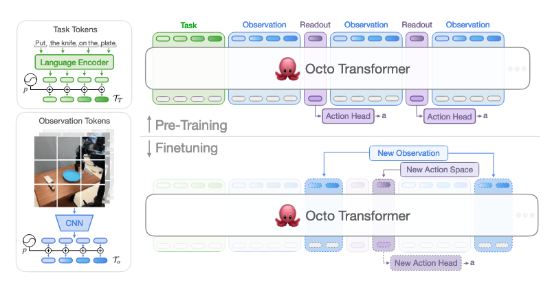
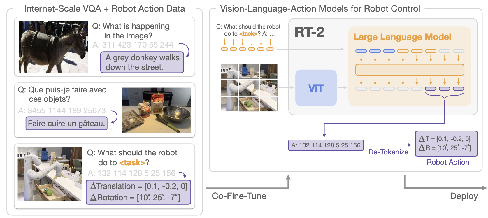
• RT-1 discretizes robot actions into 256-bin tokens, creating a shared "action language" across robots.
• It absorbs heterogeneous data from simulation and other robot morphologies without losing performance.
• It generalizes robustly to new tasks, environments, and long-horizon scenarios (up to 50 steps).

Introduction & Motivation​

• Leveraging large, diverse, task-agnostic datasets enables high performance in zero-shot or small task-specific settings.
• Data collection and curation is a critical bottleneck in robotics ("the unsung hero" of large-scale ML).
• Transformer-based controllers are powerful but inefficient for real-time robotics, requiring architectural adaptations.

Model & Architecture​

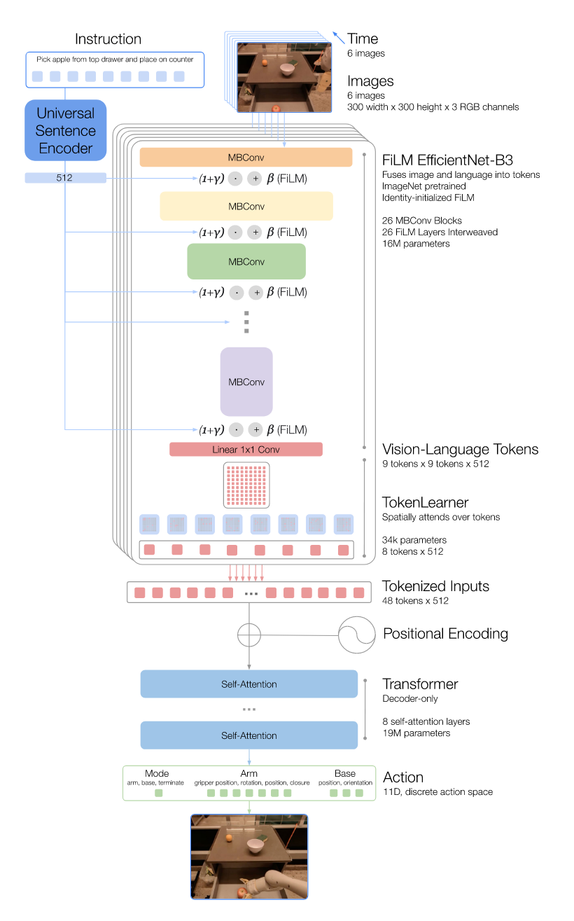
• RT-1 architecture: EfficientNet + FiLM layers + TokenLearner for compact vision-language tokenization.
• Action tokenization: 11 action dimensions (7 arm, 3 base, 1 mode) discretized into 256 bins each.
• This abstraction converts continuous robot actions into a discrete "token language", enabling cross-domain and cross-robot transfer.
• Real-time feasibility: optimized design achieves ~3Hz inference speed suitable for real-world control.

Experiments & Results​

General Performance​

• RT-1 executes over 700 unique instructions at 97% success rate.
• On unseen instructions: 76% success, outperforming next-best baseline by +24%.
• Robustness: 83% success with distractors, 59% with background changes (significantly higher than baselines).

Absorbing Simulation Data​

• Adding sim data does not degrade real-task performance.
• Objects/tasks only seen in simulation: performance boosted 23% ⇒ 87%.
• Unseen instructions with sim objects: 7% ⇒ 33%, showing strong sim-to-real domain transfer.

Absorbing Multi-Robot Data​

• Mixed RT-1 + Kuka datasets: only 2% drop in original tasks.
• Bin-picking eval: RT-1 only 22% ⇒ mixed training 39% (almost 2×).
• Kuka-only training: 0% on EDR robots ⇒ morphology transfer alone fails.
• Mixed data enables RT-1 to leverage cross-robot experiences without explicit demonstrations.

Long-Horizon Scenarios (SayCan Integration)​

• Evaluated in two kitchens:
  • Kitchen1: 67% execution success.
  • Kitchen2 (novel environment): also 67% execution success.
• Outperforms Gato (0% in Kitchen2) and BC-Z (13% in Kitchen2).
• Demonstrated execution of ultra-long tasks up to 50 steps.

Data Quantity vs Diversity​

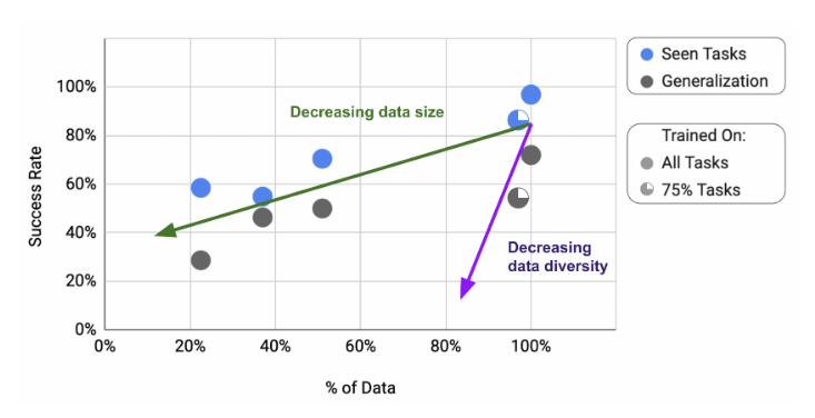
• Reducing dataset size ⇒ gradual performance/generalization decline.
• Reducing task diversity ⇒ much sharper decline, especially in generalization.
• Key takeaway: Data diversity is more critical than data quantity.

Conclusions & Limitations​

• RT-1 proves large-scale data absorption and strong generalization in robotics.
• Limitations:
  • Based on imitation learning ⇒ cannot surpass demonstrator performance.
  • Generalization limited to recombinations of known concepts ⇒ fails on truly novel motions.
  • Dataset is large but not dexterous (fine manipulation limited).

Future Directions​

• Enable non-experts to collect training data and prompt models for faster skill scaling.
• Increase environmental diversity to strengthen robustness to backgrounds/environments.
• Improve reaction speed and context retention via scalable attention and memory.

Ref​

• Brohan, A., Brown, N., Carbajal, J., Chebotar, Y., Dabis, J., Finn, C., Gopalakrishnan, K., Hausman, K., Herzog, A., & Hsu, J. (2022). Rt-1: Robotics transformer for real-world control at scale. arXiv preprint arXiv:2212.06817.

Say Can​

• The core of SayCan is using an LLM to decompose high-level instructions into low-level skills, and reinforcement-learned affordance value functions to evaluate whether each skill is feasible in the current environment.
• The Say × Can structure is modular: different LLMs or affordance models can be swapped in, but each module’s inherent biases are carried into the system.
• To mitigate limitations, loop-based strategies are essential — CoT and RLHF provide feedback loops for LLMs, while closed-loop feedback enables affordance functions to adapt during execution.

Motivation (Why LLMs alone fall short)​

• LLMs lack embodiment. They haven’t acted in the physical world, so using them for decision-making on a specific robot is unreliable.
• LLMs don’t know robot’s abilities or state. They may split instructions into subtasks, but without context of capabilities and environment, plans can be irrelevant.
• Prompting alone isn’t enough. Structured prompts help, but they don’t guarantee admissible or executable steps.

Core Proposal (What SayCan adds)​

• Ground with pretrained skills. Constrain LLM to propose actions that the robot can actually perform in context.
• Say × Can factorization.
  • Say (task-grounding): LLM estimates relevance of each skill to the instruction.
  • Can (world-grounding): Affordance functions estimate probability of success from current state.

Probabilistic Formulation​

• Two probabilities multiplied:
  • $p(\ell_\pi|i)$: LLM score of relevance.
  • $p(c_\pi|s,\ell_\pi)$: affordance score of success.
  • Select: $\pi = \arg\max p(c_\pi|s,\ell_\pi)\,p(\ell_\pi|i)$.

Planning Procedure​

• Planning is structured as a dialog: user gives high-level instruction, LLM produces a step sequence, loop until "done."
• Benefit: Interpretability—scores provide transparency.
• Caveat: Without affordances, chosen steps may be irrelevant to the current scene.

Affordances via RL​

• Affordance = value function. In sparse reward settings, value ≈ success probability.
• TD RL and MDP formalism used to learn $Q_\pi(s,a)$.

Implementation​

• Skill training:
  • BC-Z (behavioral cloning) and MT-Opt (reinforcement learning).
  • Multi-task BC/RL amortizes training cost.
• Language conditioning: Pretrained sentence encoder frozen, text embeddings as input.
• Action space: 6-DoF end-effector, gripper open/close, base x-y & yaw deltas, terminate.

Metrics​

• Plan success rate: 2/3 human raters agree that the plan is valid.
• Execution success rate: 2/3 raters agree robot achieved the task.

Key Results​

• Grounding nearly doubles performance vs non-grounded baselines.
• Understands sequence order (approach → pick → bring).
• Failures: Long-horizon tasks (early termination), negation, ambiguous references.
• Error split: ~65% LLM, 35% affordance.

Ablations​

• Remove LLM (task-grounding):
  • BC-NL: 0% all tasks.
  • BC-USE: 60% on single primitives, 0% otherwise.
• Remove affordances (world-grounding):
  • No-VF: 67%, Generative: 74% vs 84% (SayCan).

Scaling & Models​

• PaLM > FLAN. PaLM-SayCan achieves 84% plan / 74% execute.
• Stronger LMs improve robotics performance.

Extensibility​

• Add new skills easily: register skill, affordance, prompt example.
• Chain-of-Thought: Add "Explanation" → helps with negation and reasoning-heavy queries.
• Multilingual: Almost no performance drop (English, Chinese, French, Spanish).

Open-Source Variant​

• CLIPort for pick-and-place.
• Affordances approximated by ViLD open-vocabulary object detector.
• GPT-3 as language model.

Limitations & Future Work​

• Limits: Inherits LLM biases; skill library is bottleneck; hard to react to skill failures.
• Closed-loop extensions: Huang et al. use environment feedback + inner monologue for replanning.
• Future directions: Expand/robustify skills, explore new grounding sources (non-robotic), test if natural language is the right ontology, combine planning + language, use LMs for policy pretraining.

Ref​

• ichter, b., Brohan, A., Chebotar, Y., Finn, C., Hausman, K., Herzog, A., Ho, D., Ibarz, J., Irpan, A., Jang, E., Julian, R., Kalashnikov, D., Levine, S., Lu, Y., Parada, C., Rao, K., Sermanet, P., Toshev, A. T., Vanhoucke, V., Xia, F., Xiao, T., Xu, P., Yan, M., Brown, N., Ahn, M., Cortes, O., Sievers, N., Tan, C., Xu, S., Reyes, D., Rettinghouse, J., Quiambao, J., Pastor, P., Luu, L., Lee, K.-H., Kuang, Y., Jesmonth, S., Joshi, N. J., Jeffrey, K., Ruano, R. J., Hsu, J., Gopalakrishnan, K., David, B., Zeng, A., & Fu, C. K. (2023). Do As I Can, Not As I Say: Grounding Language in Robotic Affordances Proceedings of The 6th Conference on Robot Learning, Proceedings of Machine Learning Research. https://proceedings.mlr.press/v205/ichter23a.html

Data Preparation​

• In real world applications, data can be inconsistent, incomplete, and noisy.
• Data Collection problems: when data is collected incorrectly
• Incomplete Data: when information is missing
• Data entry problems: when data is entered incorrectly
• Contradictions in data: when the data says something in one place, and then says a different thing elsewhere in the dataset. We can think of this data as noisy.
• Discrepancy in naming conventions: when data descriptions are unclear, people may misinterpret their meaning.
• Duplicated records: when integrating data from different sources, the same data may get entered multiple times.
• Data transmission problems: when data is sent between different people or databases or companies, things can get lost in the process.

Data mining tasks​

• Classification
• Estimation
• Prediction
• Characterisation
• Discrimination
• Affinity grouping
• Clustering
• Time series analysis

Data Cleaning​

• Missing data
  • Ignore the record
  • Fill the missing value manually
  • Fill missing values with calculated values
    • The missing values can be filled using the average value for a particular attribute
    • or by using attribute mean for all samples belonging to the same class as the given record.
    • also be filled using methods such as Bayesian classification or decision trees to automatically infer the values.
• Noisy data: a meaningless variation that cannot be interpreted properly by machines
  • Binning
    • binning methods use the neighbour's data, this is referred to as local smoothing
    • can replace all data in a segment by its mean or boundary values
  • Clustering
    • grouping of data points according to a distance measure
    • use a clustering algorithm to classify each data point into a specific group
    • can detect outliers
  • Regression
    • a data mining function that deals with the prediction of a continuous value rather than a class
    • maps data values to a function
    • Using regression to fit data by finding a mathematical equation may be used to smooth noisy data.

Binning​

• Equi-width: Bins have equal width.
• Equi-depth: Bins have the same number of values in them or almost the same number if they don't divide equally.

Equi-width binning​

Equal-interval binning, split the whole range of numbers into intervals with equal size.

• Price: 4, 8, 9, 15, 21, 21, 22, 26, 27, 28, 29, 36
• Equal-width binning
  • Bin1 [4, 12]: 4, 8, 9
  • Bin2 (12, 20]: 15
  • Bin3 (20, 28]: 21, 21, 22, 26, 27, 28
  • Bin4 (28, 36]: 29, 36
• Smoothing by bin means
  • Bin1: 7, 7, 7
  • Bin2: 15
  • Bin3: 24, 24, 24, 24, 24, 24
  • Bin4: 33, 33
• Smoothing by bin boundaries
  • Bin1: 4, 9, 9
  • Bin2: 15
  • Bin3: 21, 21, 21, 28, 28, 28
  • Bin4: 29, 36

Equi-depth binning​

Equal-frequency binning, use intervals containing an equal number of values.

• Price: 4, 8, 9, 15, 21, 21, 22, 26, 27, 28, 29, 36
• Equal-depth binnning
  • Bin1: 4, 8, 9
  • Bin2: 15, 21, 21
  • Bin3: 22, 26, 27
  • Bin4: 28, 29, 36
• Smoothing by bin means: each value in a bin is replaced by the mean value of the bin.
  • Bin1: 7, 7, 7
  • Bin2: 19, 19, 19
  • Bin3: 25, 25, 25
  • Bin4: 31, 31, 31
• Smoothing by bin boundaries: each bin value is replace by the closest boundary value.
  • Bin1: 4, 9, 9
  • Bin2: 15, 21, 21
  • Bin3: 22, 27, 27
  • Bin4: 28, 28, 36

Data Integration​

provides unified data by combining data from various heterogeneous data sources into a coherent data store

• The sources can include flat files, databases or multiple data cubes.
• Careful integration may help to avoid and reduce inconsistencies and redundancies in the final dataset.
• Building an enterprise's data warehouse is considered one of the most popular data integration implementations.
• Redundant attributes: An attribute (feature or column of a dataset) is called redundant if it can be derived from any other attribute or set of attributes.
  • In the process of data integration in data mining, the use of multiple data stores may lead to the problem of redundancy in data.
  • Dimension naming or inconsistencies in an attribute can also lead to redundancies in the dataset.

Pearson correlation coefficient​

• Correlation analysis can be used to detect redundancies in Numerical data
• It can measure how strongly one attribute implies the other on the basis of the available data.
• > 0.5: a strong positive correlation, A⬆️ B⬆️
• < -0.5: a strong negative correlation, A⬆️ B⬇️
• 0: no correlation. A and B are independent.
• correlation != causation

$r_{A,B} = \frac{n\sum{}xy - (\sum{}x)(\sum{}y)} {\sqrt{(n\sum_{} x^2 - (\sum_{} x)^2) \, (n\sum_{} y^2 - (\sum_{} y)^2)}}$

$r_{A,B} = \frac{\sum_{} (x_i - \bar{x})(y_i - \bar{y})}{\sqrt{\sum_{} (x_i - \bar{x})^2} \, \sqrt{\sum_{} (y_i - \bar{y})^2}}$

• step-by-step derivation
  • 분산: $Var(X) = \frac{1}{n} \sum_{} (x_i - \bar{x})^2$
  • 공분산: $Cov(X,Y) = \frac{1}{n} \sum_{} (x_i - \bar{x})(y_i - \bar{y})$
  • 상관계수 (정규화): $\rho = \frac{\mathrm{Cov}(X,Y)}{\sigma_X \sigma_Y}$
  • 평균: $\bar{x} = \frac{1}{n} \sum_{}x_i \quad \bar{y} = \frac{1}{n} \sum_{} y_i$
  • 분자 전개
    • $\sum_{} (x_i - \bar{x})(y_i - \bar{y})$
    • $\sum_{} (x_i y_i - x_i \bar{y} - y_i \bar{x} + \bar{x}\bar{y})$
    • $\sum_{} (x_i y_i ) - \bar{y}\sum_{} x_i - \bar{x}\sum_{} y_i + n\bar{x}\bar{y}$
    • 평균 대입
      • $\sum_{}x_iy_i - \frac{1}{n}(\sum_{}y_i)(\sum{}x_i) - \frac{1}{n}(\sum{}x_1)(\sum{}y_1) + \frac{1}{n}(\sum{}x_1)(\sum{}y_1)$
      • $\sum{}x_iy_i - \frac{1}{n}(\sum{}x_i)(\sum{}y_i)$
  • 분모 전개
    • $\sqrt{\sum_{} (x_i - \bar{x})^2} \, \sqrt{\sum_{} (y_i - \bar{y})^2}$
    • $\sqrt{\sum_{} x_i^2 - 2\bar{x}\sum_{} x_i + n\bar{x}^2} \, \sqrt{\sum_{} y_i^2 - 2\bar{y}\sum_{} y_i + n\bar{y}^2}$
    • 평균 대입
      • $\sqrt{\sum_{} x_i^2 - \frac{2}{n}(\sum_{} x_i)(\sum_{} x_i) + \frac{1}{n}(\sum{}x_i)^2} \, \sqrt{\sum_{} y_i^2 - \frac{2}{n}(\sum_{} y_i) + \frac{1}{n}(\sum{}y_i)^2}$
      • $\sqrt{\sum_{} x_i^2 - \frac{1}{n}(\sum_{} x_i)^2} \, \sqrt{\sum_{} y_i^2 - \frac{1}{n}(\sum_{} y_i)^2}$
  • 재정의 $r_{A,B} = \frac{\sum{}x_iy_i - \frac{1}{n}(\sum{}x_i)(\sum{}y_i)} {\sqrt{(\sum_{} x_i^2 - \frac{1}{n}(\sum_{} x_i)^2) \, (\sum_{} y_i^2 - \frac{1}{n}(\sum_{} y_i)^2)}}$
  • 분자/분모에 n 곱하고 인덱스 생략 $r_{A,B} = \frac{n\sum{}xy - (\sum{}x)(\sum{}y)} {\sqrt{(n\sum_{} x^2 - (\sum_{} x)^2) \, (n\sum_{} y^2 - (\sum_{} y)^2)}}$

Data Transformation​

The data is consolidated or transformed so that the patterns found are easier to understand, and the consequent mining process is more efficient.

• Smoothing: smoothing is used to remove noise from the data to improve clarity around the important features in the dataset
• Normalization: the method of scaling your data, into a regularized range, so that you can compare and represent it more accurately
• Discretization & Concept hierarchy generation
  • Discretisation is the process of putting values into buckets so that there are a limited number of possible states.
  • Discretisation transforms a continuous attribute into a categorical attribute, usually happens after the data is cleaned.
  • This process includes replacing lower-level data (primitive) with higher-level concepts through the use of concept hierarchies.
  • Street may be replaced with city, country or region.
  • Age may be replaced with senior, adult, younger and youth.
• Binarization: transforming data into binary numbers (e.g. 0, 1).
  • This helps make classifier algorithms more efficient.

Data Nomalization​

• the data should be standardised or normalised in order to avoid dependency on the selection of measurement units.

• This constitutes transforming data to lie within a common or smaller range, like [0.0, 1.0] or [−1, 1].

• Min-max normalization

  • Min-max normalisation maps a value of $K$, indicated by $v_n$, to a new value $v'_n$ within the range $[new\_min_K, new\_max_K]$
    • $v'_n = \frac{(v_n - min_K)}{(max_K - min_K)} \cdot (new\_max_K - new\_min_K) + new\_min_K$
    • calculates the relative position within the original range and reflects it in the new range accordingly.
  • preserves the relationships between the original data values.
  • It will encounter an out-of-bounds error if a future input case for normalisation falls outside of the original data range for K.

• Z-Score normalization

  • normalises attribute values using the average (i.e., mean) and standard deviation of $K$.
    • $v'_n = \frac{(v_n - \mu_K)}{\sigma_K}$
    • It converts the distance of a data point from the mean into a unitless measure.
  • is useful when there are outliers that dominate the min-max normalisation
  • is useful when the actual minimum and maximum of attribute $K$ are unknown.

• Decimal scaling normalization

  • The number of decimal points moved is based on the maximum absolute value of $K$.
    • $v'_n = \frac{v_n}{10^j}$
    • where $j$ is the smallest integer such that $max(|v'_n|) < 1$.
    • divides all values by the power of 10 just larger than the maximum absolute value, bringing them into the range $(-1, 1)$.

• Softmax normalization

  • a nonlinear transformation that yields an 's'-shaped curve that approaches 0 and 1 asymptotically.
  • New values will be mapped between 0 and 1 even if they are beyond the range of your existing data.
  • $\alpha = \frac{\nu - \mu}{\lambda \, (\sigma / 2\pi)}, \qquad \nu' = \frac{1}{1 + e^{-\alpha}}$
    • Center the data around the mean :: use $(\nu - \mu)$
    • Remove units by scaling with the standard deviation :: divide by $\sigma$.
    • Control how steep or flat the curve is :: adjust with $\lambda$.
    • Add $(2\pi)$ as a conventional constant to better match the logistic curve with statistical distributions.
    • the formula naturally arises by centering at the mean, standardizing by the spread, letting the user control the slope, and refining with a scaling constant.

• Sigmoid normalization

  • a nonlinear transformation similar to softmax. It ranges between −1 and 1 (asymptotically), and has a fixed linear portion within $±mu$.
    • $\alpha = \frac{\nu - \mu}{\lambda \, (\sigma / 2\pi)}, \qquad \nu' = \frac{1 - e^{-\alpha}}{1 + e^{-\alpha}}$
    • Center the data around the mean :: use $(\nu - \mu)$
    • Remove units by scaling with the standard deviation :: divide by $\sigma$.
    • Control how steep or flat the curve is :: adjust with $\lambda$.
    • Add $(2\pi)$ as a conventional constant to refine scaling with respect to statistical distributions. Apply the hyperbolic tangent :: map the result smoothly into the range $[-1, 1]$.
    • the formula naturally arises by centering at the mean, standardizing by spread, letting the user control the slope, and using tanh to compress all values into $[-1, 1]$.

Discretization & Concept hierarchy generation​

• Data discretisation is a form of numerosity reduction that transforms a continuous attribute into a categorical attribute.
• Higher concept labels or a smaller number of intervals (i.e. binning) are used to replace the raw data in order to simplify the original data and increase the efficiency of mining.
• Discretisation is very beneficial for generating concept hierarchies automatically, which allow data mining at multiple levels of data abstraction.
• One or more concept hierarchy can be defined for the single attribute for accommodating the requirements of various users.

• If dependent and independent variables have only a few values, a wide range of classification algorithms can be used.

Data Binarizaion​

• maps a categorical or continuous attribute into one or more binary variables.
• Binarisation can convert a continuous attribute to a categorical attribute which can then be converted into set of binary attributes.
• only possible to keep the meaning of one categorical value at one time, losing the meaning of the others.

Data Reduction​

• to acquire a reduced data set representation which is much smaller in quantity and maintains the quality of the data close to the original data.
• to reduce data storage and analysis costs while increasing storage efficiency

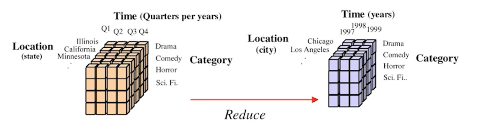
Aggregation​

• storing and presenting data as a summary, using statistical metrics like means, median and variance.
• Data aggregation is often used to construct a data cube for data analysis at multiple levels of abstraction.
• Multidimensional aggregated information is stored in data cubes

Dimensionality reduction​

• to minimize the number of features
• feature subset selection or feature selection detects and removes weakly relevant, redundant, or irrelevant dimensions or attributes
• to determine a minimum set of attributes so that the resulting probability distribution of the data classes is as near as possible to the original distribution obtained using all attributes.
• Feature subset selection: uses only available subsets of the features to reduce the dimensionality of the data
  • Redundant features: Duplicates of all or much of the information present in one or more attributes.
    • the amount of sales tax paid / purchase price of a product
  • Irrelevant features: Contain no information that is important for the data mining process at hand.
    • the color of a product when predicting its price
  • While some redundant and irrelevant attributes can be eliminated immediately by considering the domain knowledge or common sense.
  • The ideal approach to feature selection is to try all possible subsets of features in the input for the data mining algorithm of interest, and then consider the subset that gives the best outcome.
• Feature subset selection techniques
  • Brute-force approach
  • Embedded approaches:
    • Feature selection occurs naturally as part of the data mining algorithm.
    • The algorithm decides by itself which attributes are to be ignored.
  • Filter approaches:
    • Features are chosen before running the data mining algorithm by taking some of the approaches which are independent of the data mining process.
    • can be selected with pairwise correlation as low as possible.
  • Wrapper approaches:
    • consider the target data mining algorithm as a black box to determine the best subset of attributes.
    • Instead of evaluating all possible combinations, it intelligently searches only a subset to find a near-optimal feature set.
    • Heuristic methods: Forward selection, backward elimination, genetic algorithm, greedy search.
    • Decision tree induction

Numerosity reduction​

• Regression, clustering, histograms, sampling
• reducing the volume of the data, without any loss of data
  • parametric models: store only the model parameters rather than the actual data, regression, log-linear models
  • non-parametric approaches: clustering, sampling, histograms
• Histograms
  • unsupervised techniques that does not use a class label
  • Singleton bucket: each of the buckets shows only a single frequency pair/attribute value
  • Equal-width histogram: divided into equal ranges
  • Equal-frequency(depth) histogram: each bucket has the similar number of data
• Sampling
  • a large dataset to be denoted by a smaller random subset (or sample) of the data
  • often used in preliminary exploration as well as final analysis.
  • useful when processing the entire dataset is too large or expensive.
  • If the sample preserves the important properties of the original dataset (e.g., the mean), the sample is said to be representative
  • Simple random sampling: every data point has an equal probability of being chosen.
  • Sampling without replacement: once a data point is chosen, it cannot be selected again.
  • Sampling with replacement (bootstrap): the same data point can be picked multiple times, since it is placed back into the dataset after selection.
  • Cluster sampling: the dataset is divided into clusters (groups), and sampling is performed at the cluster level.
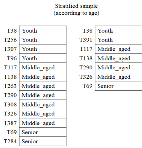
  • Stratified sampling: the dataset is split into strata (partitions), and random samples are drawn from each stratum. This is especially useful when the data is imbalanced, e.g., sampling customers across different age groups.

• Strata: Youth, Middle-aged, Senior

Vocabulary & Expressions​

Key Idea​

• CLIPort proposes a two-stream architecture for vision-based manipulation:
  • Semantic pathway (what): leverages CLIP for broad semantic understanding.
  • Spatial pathway (where): leverages Transporter for fine-grained spatial reasoning.
• This design is inspired by the two-stream hypothesis in cognitive psychology (ventral/dorsal pathways).

Framework Contributions​

• Benchmark Extension: Expanded the Ravens benchmark with language-grounding tasks for manipulation.
• Two-Stream Architecture: Uses pre-trained vision-language models (CLIP) to condition precise manipulation policies with language goals.
• Empirical Results: Demonstrates robustness on diverse manipulation tasks, including multi-task settings and real-robot experiments.

Architectural Design​

• CLIPort integrates semantic (CLIP) with spatial (Transporter) features by lateral fusion.
• The semantic stream is conditioned with language features from CLIP’s text encoder and fused with intermediate spatial features.
• Enables end-to-end learning of affordance predictions (pick-and-place) without explicit object models, segmentations, or symbolic states.

Key Insights​

• Formulates manipulation as action detection (where to act), instead of object detection.
• Tabula rasa systems (like plain Transporter) require new demonstrations for every goal/task. CLIPort addresses this with a strong semantic prior (from CLIP) to generalize across tasks and concepts.
• Language-conditioned policies provide an intuitive interface for specifying goals and transferring concepts.

Experimental Results​

• Simulation (PyBullet, UR5 robot with suction gripper):
  • 10 language-conditioned tasks with thousands of unique instances.
  • Multi-task CLIPort outperformed or matched single-task models, even with fewer demonstrations.
  • CLIP-only or Transporter-only baselines saturate, while CLIPort exceeds 90% success with just 100 demos.
• Generalization:
  • CLIPort generalizes to unseen attributes (e.g., new colors, shapes, object categories).
  • Struggles with completely novel attributes (e.g., “pink” or “orange” never seen in training).
• Real-World Robot Experiments (Franka Panda):
  • Achieved ~70% success on real tasks with just 179 demonstrations.
  • Performance trends were consistent with simulation, validating sim-to-real transfer.

Conclusion​

• CLIPort shows that multi-task, language-conditioned policies generalize across tasks better than object-centric or tabula rasa methods.
• With action abstraction and spatio-semantic priors, end-to-end models can learn new skills without requiring hand-engineered pipelines.
• Limitations remain for dexterous 6-DoF manipulation and complex continuous control.

Ref​

• Shridhar, M., Manuelli, L., & Fox, D. (2022). Cliport: What and where pathways for robotic manipulation. Conference on robot learning.

Overview​

• Introduces a HoOA benchmark that isolates hallucinations on object attributes (color, shape) from existence/relationship errors.
• Proposes MIAVLM: leverages multiview images (generated from a single image’s 3D representation) and a Multiview Attributes Perceiver (MAP) to make fusion order-invariant.
• Adds negative instructions during tuning to counter LVLMs’ tendency to answer "Yes".
• Results: best HoOA metric (0.775 / 0.787) with fastest inference (0.071 / 0.105 s). "9in1" tiling is ineffective; separate multiview inputs help.
• Training: LM loss, Adam (lr=0.001), cosine annealing, 20 epochs, single NVIDIA 3090.

Hallucinations on Object Attributes (HoOA)​

Issues​

• HoOA = incorrect attribute descriptions for existing objects (distinct from HoOE/HoOR).
• Root causes analyzed:
  • Single-view insufficiency: fine-grained details can be invisible from a single viewpoint.
  • Instruction bias: overexposure to positive/affirmative patterns → "Yes" bias.
  • Order sensitivity: multi-image inputs change predictions when view order changes.

Mitigation Methods (this paper)​

• Multiview prompts: sample views from a single image’s 3D reconstruction to recover missed details.
• MAP (order-invariant fusion): learn view weights and fuse per-view features via weighted sum; input order has no effect; supports any number of views.
• Negative instructions: incorporate "No"-answerable questions in tuning to suppress "Yes" bias.

Benchmark (HoOA)​

Construction​

• Based on CelebAText-HQ; manual attribute descriptions rewritten into Yes/No questions.
  • Positive questions → correct answer "Yes".
  • Negative questions → attribute flipped/opposite → correct answer "No" (to expose "Yes" bias).
• Scale: 1,430 images, 14,291 positive + 14,291 negative questions.
• Split: 9:1 train:test.
• Metric: average of accuracy on positive and negative questions (balanced HoOA score).

Model: MIAVLM​

Visual Extractor (VE)​

• 6 stacked Transformer decoder blocks.
• Soft prompts $P \in \mathbb{R}^{l \times d}$ are queries; image embeddings $e_i$ are keys/values.
• Per-view cross-attention computed in parallel (no autoregressive chaining; no assumed order).
• Per-view output: $$o_i = \mathrm{softmax}\!\left(\frac{(P W_Q)(e_i W_K)^\top}{\sqrt{d}}\right) e_i W_V,\quad O_{VE}=\{o_1,\dots,o_n\}.$$

Multihead Sampler (MS)​

• Learns view weights for fusion.
• Decomposer (2-layer MLP) maps each view’s $[CLS]$ to $m=4$ tokens $\{e_i^{1},\dots,e_i^{m}\}$.
• For each token/head $j$: compute attention scores vs. $P$ → mean over prompt tokens → $\mathrm{weights}^j \in \mathbb{R}^n$.
• Average across heads: $$w_{MS} = \tfrac{1}{m}\sum_{j=1}^{m}\mathrm{weights}^j \in \mathbb{R}^n.$$

MAP (Multiview Attributes Perceiver)​

• Order-invariant weighted fusion: $$\text{Output}=\sum_{i=1}^{n} w_i\,o_i.$$
• Properties: supports any number of views; permutation-invariant to input order.
• By learning weights for each view, MAP highlights informative perspectives and suppresses less useful ones, ensuring consistent predictions even when the view order changes. This directly addresses the input-order sensitivity observed in baselines such as OpenFlamingo.

Benchmarks​

Baselines & Input Modes​

• Baselines: BLIP3, OpenFlamingo (4 variants), OPERA, Idefics2, LLaVA-UHD.
• Two input modes:
  1. Original image only.
  2. Original + 8 generated views.
     • Models that accept only one image use 9in1 tiling (nine images stitched into one).

Main Results​

• MIAVLM:
  • HoOA metric: 0.775 / 0.787 (modes 1 / 2)
  • Positive accuracy: 0.752 / 0.762
  • Negative accuracy: 0.797 / 0.812
  • Inference time: 0.071 / 0.105 s (fastest)
• 9in1 tiling did not improve results (likely harder to interpret).
• Nine separate multiview images generally improved performance.

Ablations​

• Negative instructions: boost negative-question accuracy but slightly reduce positive-question accuracy; overall HoOA increases (approx. 0.665 → 0.787).
• Input-order sensitivity:
  • MIAVLM is order-invariant
  • OpenFlamingos accuracy varies when shuffling view order.

Limitations & Notes​

• Trade-off from negative instructions (negatives ↑, positives ↓).
• Effectiveness depends on the quality of generated views.

Insights​

• This approach seems especially suitable for perception, where multiple scene views may arrive in arbitrary order, ensuring consistent attribute recognition.

Ref​

• Tan, Z., Li, Y., Meng, S., Yuan, X., Li, W., Mo, T., Wang, B., & Chu, X. (2025, 6–11 April 2025). Mitigating Hallucinations on Object Attributes using Multiview Images and Negative Instructions. ICASSP 2025 - 2025 IEEE International Conference on Acoustics, Speech and Signal Processing (ICASSP).

match​

match term:
  case pattern-1:
    action-1
  case pattern-2:
    action-2
  case pattern-3:
    action-3
  # the underscore _ case executes the default code
  case _:
    action-default

Repetition Statements​

• The count-controlled repetition: a fixed number of times.
• The sentinel-controlled repetition: a designated value that ends the loop.
• The infinite repetition: continues until externally stopped.

The For Loop​

for <value> in <range of values>:
  <code>

sum = 0;

# [1, 2, ..., 19]
# adds values from 1 to 19 to sum
for e in range(1, 20):
  sum += e

print(f"The sum is: {sum}")

Loop-And-A-Half​

n = 5
sum = 0

while n < 10:
  sum += n

  if sum > 100:
    break

동기화 설정​

Settings - Sync - Data Syncing

• 로그인하고 자동 동기화 설정

브라우저 익스텐션 다운로드​

• Zotero Connector

Citation 설정​

Settings - Cite - APA 7th

• 등록되어있는지 확인

Export - Item Format - APA 7th

• 포맷 설정

MS Word Plugin 설치​

Settings - Cite - Word Processors

• Microsoft Word 섹션의 Install/Reinstall Microsoft Word Add-in 클릭
• 워드 재시작

플러그인 설치​

Tools - Plugins

• 다운로드 받은 플러그인 드래그 앤 드랍

VSCode 플러그인​

• 아직 못 찾음

Overview​

• Mitigates exposure of private data, produces harmful outputs, or is vulnerable to attacks.
• SOTA models: LLaVA, Flamingo, GPT-4

Privacy​

Privacy Issues​

• risk escalates significantly with relevant images as optimizing in the pixel domain is easier than in text
• can unintentionally memorize sensitive data, leading to leaks without knowledge of the model’s specifics
• Overfitting may also cause retention of sensitive attributes during inference
• gradient-based and backdoor attacks further jeopardize VLM privacy with open-source data

Privacy Mitigation Methods​

• New metrics have been created to assess a model’s ability to reproduce training instances and facilitate cross-model comparisons
• models utilizing multiple modalities provide better privacy
• safety modules can be integrated to boost resilience against violations
• adversarial training can enhance privacy but risks reducing accuracy
• New architecture: differentially private CLIP model

Privacy Future Research Directions​

• Cryptography-based Privacy Preservation
  • Secure multi-party computation (SMPC): divides secret information into shares among multiple parties, ensuring that individual shares reveal nothing unless combined
  • Homomorphic encryption (HE): allows computations on encrypted data without decryption, and has also been utilized for privacy preservation in transformers
• Federated Learning
  • enhances privacy in vision-language models (VLMs) by localizing model training, which protects training data from leakage.
  • challenges such as communication overhead among devices and statistical heterogeneity from diverse data distributions
• Data Manipulation and Finetunning
  • Data pseudonymization: substitutes sensitive information with synthetic alternatives.
  • Data Sanitization: removes duplicates to reduce memorization and privacy risks.
  • knowledge sanitization-fine-tuning: provide safe responses when leakage risks arise.

Fairness and Bias​

Fairness and Bias Issues​

• Bias from training data
  • disproportionately features men and lighter-skinned individuals
  • outdated vocabulary and imbalanced representation
  • clinical models may favor certain patient groups based on gender, language, etc.
• Bias from Model
  • Gender biases
  • misclassification of race-related elements and biased outputs

Fairness and Bias Mitigation Methods​

• New Datasets and Benchmarks
  • Harvard-FairVLMed, PATA, and BOLD enhance evaluations but often lack the scale of established benchmarks.
  • create synthetic datasets to improve fairness assessments
    • gender-balanced dataset generated with DALL-E-3 and another consisting of gender-swapped images
    • counterfactual image-text pairs that highlight biases in datasets like COCO Captions
  • new metrics
    • gender polarity
    • bias distance in embeddings
  • human evaluation
• De-biasing
  • adjust model instructions and architectures for improved fairness
  • detecting biased prompts in pre-trained models
  • Post-hoc Bias Mitigation (PBM) effectively reduce bias in image retrieval
  • Re-sampling underperforming clusters can enhance fairness
  • modification of facial features also mitigate biases
  • self-debiasing reduces biased text generation, especially when paired with other methods

Fairness Future Research Directions​

• Optimized De-biasing
  • Additive residual learning: for fairer image representations.
  • Calibration loss: retain semantically similar embeddings.
  • Counterfactual inference framework: help models learn correct responses through cause and effect.
  • Adversarial classifiers: predict image attributes from visual-textual similarities can be combined with instruction tuning to reduce bias.
• Disentangled Representation Learning (DRL): simplifies complex data by breaking it in to independent feature groups, improving model predictions.
  • Traditional DRL
    • Variational autoencoders (VAEs) for feature encoding based on impact
    • Generative adversarial networks (GANs) for separation.
  • Attention in text encoders can be adjusted for fairer outputs.
  • challenges: varying definitions of "disentanglement", ensuring fairness.
• Human-in-the-Loop (HITL): integrating human intervention into their training to improve precision and fairness
  • active learning
  • reinforcement learning with human feedback
  • explainable AI
  • challenges: human bias, finance, and ethical and legal issues persist

Robustness​

Robustness Issues​

• Out-of-Distribution (OOD) Robustness
  • ChatGPT excels in adversarial tasks but struggles with OOD robustness and informal medical responses
  • MLLMs often fail to generalize beyond training domains due to mapping issues
  • vision-language models face difficulties with open-domain concepts, especially when overfitting during fine-tuning
  • Large pre-trained image classifiers show initial robustness, which diminishes over time
  • Current visual question answering (VQA) models are limited to specific benchmarks, hindering generalization to OOD datasets
  • fine-tuning may impair model calibration in OOD contexts.
• Adversarial Attack Robustness
  • Studies indicate that open-sourced VLMs show performance gaps in red teaming tasks, highlighting the need for improved safety and security.
  • misalignment between language and vision modalities creates a "modality gap", complicating adversarial vulnerability.

Robustness Mitigation Methods​

• Improving Out-of-Distribution Robustness
  • enhance OOD detection and generalization. A simple maximum logit detector has been shown to outperform complex methods for anomaly segmentation
  • In-context learning (ICL) can also improve multimodal generalization
  • A fine-tuned CLIP excels in unsupervised OOD detection
  • The OGEN method synthesizes OOD features
  • Maximum Concept Matching aligns visual and textual features, and anchor-based finetuning leads to better domain shifts
• Defense Against Adversarial Attacks
  • VILLA is a two-stage framework for adversarial training of VLMs, featuring task-agnostic adversarial pre-training and task-specific finetuning
    • conducts adversarial training in the embedding space rather than on raw image pixels and text tokens, improving the model’s resilience against adversarial examples
    • SOTA performance across various tasks

Robustness Future Research Directions​

• Data Augmentation
  • MixGen: a data augmentation method that generates new image-text pairs by interpolating images and concatenating text to preserve semantics.
  • creating synthetic images involves extracting text prompts via an image captioning model for use in text-to-image diffusion, then mixing these with real datasets.
  • bimodal augmentation (BiAug): decouples objects and attributes to synthesize vision-language examples and hard negatives, using LLMs and an object detector to generate detailed descriptions and inpaint corresponding images.
• Improved Cross-Modal Alignment
  • Sharing learnable parameters
  • Applying bidirectional constraints
  • Adjusting cross-modal projections
• challenges: addressing the modality gap, which impacts robustness to OOD data and adversarial examples

Safety​

Safety Issues​

• Toxicity
  • LAION-400M: contains problematic content, including explicit materials and harmful stereotypes
  • Advanced models like GeminiProVision and GPT-4V show inherent biases
  • Assigning personas to ChatGPT can increase toxicity and reinforce harmful stereotypes
• Jailbreaking Risk
  • Perturbation can be performed effectively, while FigStep converts harmful content into images with an 82.5% attack rate across multiple VLMs
  • replaces captions with malicious prompts, enabling jailbreaks.

Safety Mitigation Methods​

• Safety Fine-Tuning
  • VLGuard
  • fine-tuned on synthetic data, reducing sensitivity to NSFW inputs and enhancing performance in cross-modal tasks
• Other approach
  • Reinforce-Detoxify: uses reinforcement learning to mitigate toxicity and bias in transformer models
  • simple mitigations improve automatic scores, these methods risk over-filtering marginalized texts and create discrepancies between automatic and human judgments

Safety Future Research Directions​

• Context Awareness
  • integrating Chain-of-Thought for improved reasoning can enhance CAER tasks with Large VLMs.
  • Dual-Aligned Prompt Tuning: combines explicit context from pre-trained LLMs with implicit modeling to create more context-aware prompts
  • Visual In-Context Learning: optimizes image retrieval and summarization to enhance task-specific interactions.
• Automated Red Teaming (ART)
  • RTVLM: a dataset that benchmarks VLMs across faithfulness, privacy, safety, and fairness
  • Arondight: automates multi-modal jailbreak attacks using reinforcement learning and uncovers significant security vulnerabilities
  • GPT-4 and GPT-4V are more robust against jailbreaks than open-source models
  • limited transferability of visual jailbreak methods compared to textual ones
  • connects unsafe outputs to prompts, improving the detection of vulnerabilities in text-to-image models

Ref​

• Vu, K., & Lai, P. (2025). Trustworthiness in Vision-Language Models. In J. Kertesz, B. Li, T. Supnithi, & A. Takhom, Computational Data and Social Networks Singapore.

Overview​

Most visual recognition studies rely heavily on crowdlabelled data in DNN

• Background development of visual recognition paradigms
• Foundations its architecture
• Datasets in VLM pre-training and evaluations
• Review and categorization of existing pre-training methods
• Benchmarking analysis discussion
• Reach challenges & potential research direction
• Training hard
  • New learning paradigm
• Vision-Language Model Pre-training and Zero-shot Prediction
  • Increasing attention
• VLMs with transfer learning
  • Prompt tuning
  • Visual adaption
• VLMs with knowledge distillation
  • distill knowledge from VLMs to downstream tasks

The development of visual recognition paradigms​

• Traditional ML: Hand-crafted features for prediction.
• Deep Learning: Deep networks (e.g., ResNet) with large-scale labeled data.
• Supervised Pre-training + Fine-tuning: Learned representations transferred to downstream tasks.
• Unsupervised / Self-supervised Pre-training + Fine-tuning: Objectives like masked modeling and contrastive learning to learn representations.
• Vision-Language Models & Zero-shot: Leverage large-scale web data, enabling zero-shot prediction without task-specific fine-tuning.
  • Collecting large-scale informative image-text data
  • Designing high-capacity models for effective learning from Bigdata.
  • Designing new pre-training objectives for learning effective VLMs.

• CLIP: Image-text contrastive objective and learns by pulling the paired images and texts close and pushing others faraway in the embedding space.
  • enables effective usage of web data and allows zero-shot predictions without task-specific finetuning.

VLM Overview​

• Given Image-text pairs.
• Employs a text encoder and an image encoder to extract image and text features.
• Learns the vision-language correlation with certain pre-training objectives.
• GAP: Global Average Pooling, a technique used to reduce the spatial dimensions of feature maps while retaining important information.
• ViT: Vision Transformer: Transformers for image recognition at scale.
• CNN Based: VGG, ResNet, EfficientNet
  • ResNet: Adopts skip connections between convolutional blocks which mitigates gradient vanishing and explosion and enables DNN training.
  • ResNet-D: Replace global average pooling with transformer multi-head attention.
• Transformer Based: ViT
  • Adding a normalization layer before the transformer encoder.

VLM pre-training Objectives​

Contrastive Objectives​

• Pros
  • Enforce positive pairs to have similar embeddings in contrast to negative pairs.
  • Encourages VLMs to learn discriminative vision and language features, where more discriminative features lead to more confident and accurate zero-shot predictions.
• Cons
  • Joint optimizing positive and negative pairs is complicated and challenging.
  • Involves a heuristic temperature hyper-parameter for controlling the feature discriminability.

Image Contrastive Learning​

• Forcing a query image to be close with its positive keys (its data augmentations)
• Faraway from its negative keys (other images)
• Learn discriminative features in image modality, which often serves as an auxiliary objective for fully exploiting the image data potential.

Image-Text Contrastive Learning​

• Pulling the embeddings of paired images and texts close while pushing others away.
• Minimizing a symmetrical image-text infoNCE loss
• Learn vision-language correlation by contrasting image-text pairs.
  • CLIP: A symmetrical image-text infoNCE loss
  • ALIGN: scales up the VLM pre-training with large-scale (but noisy image-text pair with noise-robust contrastive learning)
  • DeCLIP: Nearest-neighbor supervision to utilize the information from similar pairs, enabling effective pre-training on limited data.
  • OTTER: Optimal transport to pseudo-pair images and texts reducing the required training data.
  • ZeroVL: Limited data resource via debiased data sampling and data augmentation with coin flipping mixup.
  • FILIP: Region-word alignment into contrastive learning, enabling to learn fine-grained vision-language corresponding knowledge.
  • Pyramid-CLIP: Multiple semantic levels and performs both cross-level and peer-level contrastive learning for effective VLM pre-training.
  • LA-CLIP, ALIP: LLM to augment synthetic captions for given images while RA-CLIP retrieves relevant image-text pairs for image-text pair augmentation.

Image-Text-Label Contrastive Learning​

• Supervised Contrastive Learning into image-text contrastive learning.
• Learn discriminative and task-specific features by exploiting both supervised labels and unsupervised image-text pairs.
  • UniCL: pre-training allows learning both discriminative and task-specific (image classification) features simultaneously with around 900M image-text pairs.

Generative Objectives​

• Encouraging VLMs to learn rich vision, language and vision-language contexts for better zero-shot predictions.
• Generally adopted as additional objectives above other VLM pre-training objectives for learning rich context information.

Masked Image Modelling​

• Cross-patch correlation by masking and reconstructing images.
• Learn image context information by masking and reconstructing images
  • MAE, BeiT: certain patches in an image are masked and the encoder is trained to reconstruct them conditioned on unmasked patches.

Masked Language Modelling​

• Adopted pre-training objectives in NLP.
• Randomly masking a certain percentage of input tokens and predicting them. (15% in BERT)
• Learn by masking a fraction of tokens in each input text and training networks to predict the masked tokens.
  • FLAVA: masks out 15% text tokens and reconstructs them from the rest tokens for modelling cross-word correlation.
  • FIBER: adopts masked language modelling as one of the VLM pre-training objectives to extract better language features.

Masked Cross-Modal Modelling​

• Integrates masked image modelling and masked language modelling.
• Given an image-text pair, it randomly masks a subset of image patches and a subset of text tokens and then learns to reconstruct them.
• Learn by masking a certain percentage of image patches and text tokens and training VLMs to reconstruct them based on the embeddings of unmasked image patches and text tokens.
  • FLAVA: 40% image patches and 15% text tokens as in, and employs a MLP to predict masked patched and tokens, capturing rich vision-language correspondence information.

Image-to-Text Generation​

• Generate descriptive texts for a given image for capturing fine-grained vision-language correlation by training VLMs to predict tokenized texts.
  • COCA, NLP, PaLI: train VLMs with the standard encoder-decoder architecture and image captioning objectives.

Alignment Objectives​

Align image–text pairs in the embedding space.

• pros
  • simple, easy to optimize
  • can be easily extended to model fine-grained vision-language correlation
• cons
  • little correlation information within vision or language modality.
• adopted as auxiliary losses to other VLM pre-training objectives for enhancing modelling the correlation across vision and language modalities.

Image-Text Matching​

• models the overall correlation between an entire image and an entire sentence. (전역적 상관관계)
• Image-text matching models global image-text correlation by directly aligning paired images and texts
  • FLAVA: matches the given image with its paired text via a classifier and a binary classification loss.
  • FIBER: follows to mine hard negatives with pair-wise similarities for better alignment between image and text.

Region-Word Matching​

• captures fine-grained correlations between image regions and specific words. (지역적 상관관계)
• models local fine-grained vision-language correlation by aligning paired image regions and word tokens.
• benefiting zero-shot dense predictions in object detection and semantic segmentation.
  • GLIP, FIBER, DetCLIP: replace object classification logits by region-word alignment scores.
    • the dot-product similarity between regional visual features and token-wise features.

VLM Pre-Training Frameworks​

Evaluation​

Zero-shot Prediction​

• Image Classification: classify images into pre-defined categories like "prompt engineering".
• Semantic Segmentation: by comparing the embeddings of the given image pixels and texts.
• Object Detection: localize and classify objects in images with the object locating ability learned from auxiliary datasets.
• Image-Text Retrieval
  • Text-to-image retrieval that retrieves images based on texts
  • Image-to-text retrieval that retrieves texts based on images.

Linear Probing​

• freezes the pre-trained VLM
• trains a linear classifier to classify the VLM-encoded embeddings to assess the VLM representations.

Datasets​

• For Pre-training VLMs
  • CLIP, 2021, 400M, English
  • ALIGN, 2021, 1.8B, English
  • FILIP, 2021, 300M, English
  • WebLi, 2022, 12B, 129 Languages
• For VLM Evaluation
  • Image Classification
    • PSACAL VOC 2007 Classification, 11-point mAP
    • Oxford-IIIT PETS, Mean Per Class
    • EuroSAT, Accuracy
    • Hateful Memes, ROC AUC
    • Country211, Accuracy
  • Image-Text Retrieval
    • Flickr30k, Recall
    • COCO Caption, Recall
  • Action Recognition
    • UCF101, Accuracy
    • Kinetics700, Mean(top1, top5)
    • RareAct, mWAP, mSAP
  • Object Detection
    • COCO 2017 Detection, box mAP
    • LVIS, box mAP
    • ODinW, box mAP
  • Semantic Segmentation
    • Cityscapes, Mean IoU
    • ADE20K, Mean IoU

VLM Transfer learning​

which adapts VLMs to fit downstream tasks via prompt tuning, feature adapter.

• image and text distributions gap: downstream dataset may have task-specific image styles and text formats
• training objectives gap: VLMs are generally trained with task-agnostic objectives, while downstream tasks often involve task-specific objectives. (coarse or fine-grained classification, region or pixel-level recognition)

Transfer via Prompt Tuning​

Inspired by the "prompt learning" in NLP

• pros
  • simple, easy-to-implement
  • requires little extra network layer or complex network modifications
  • adapting VLMs in a black-box manner, which has clear advantages in transferring VLMs that involve concerns in intellectual property.
• cons
  • low flexibility by following the manifold (잠재 공간) of the original VLMs in prompting.

Transfer with Text Prompt Tuning​

• Exploring more effective and efficient learnable text prompts with several labelled downstream samples for each class.
  • supervised and few-shot supervised
    • CoOp: Exploring context optimization to learn context words for a single class name with learnable word vectors.
    • CoCoOp: Exploring conditional context optimization that generates a specific prompt for each image.
    • SubPT: designs subspace prompt tuning to improve the generalization of learned prompts.
    • LASP: regularizes learnable prompts with hand-engineered prompts.
    • VPT: models text prompts with instance-specific distribution with better generalization on downstream tasks.
    • KgCoOp: enhances the generalization of unseen class by mitigating the forgetting of textual knowledge.
    • SoftCPT: fine-tunes VLMs on multiple few-shot tasks simultaneously for benefiting from multi-task learning.
    • PLOT: employs optimal transport to learn multiple prompts to describe the diverse characteristics of a category.
    • DualCoOp, TaI-DP: transport VLMs to multi-label classification tasks.
      • DualCoOp: adopts both positive and negative prompts for multi-label classification
      • TaI-DP: double-grained prompt tuning for capturing both coarse-grained and fine-grained embeddings.
    • DenseCLIP: explores language-guided fine-tuning that employs visual features to tune text prompts for dense prediction.
    • ProTeCt: improves the consistency of model predictions for hierarchical classification task.
  • unsupervised
    • UPL: optimizes learnable prompts with self-training on selected pseudo-labeled samples.
    • TPT: explores test-time prompt tuning to learn adaptive prompts from a single downstream sample.

• V is learnable word vectors that are optimized by minimizing the classification loss with the downstream samples.

Transfer with Visual Prompt Tuning​

• Transfers VLMs by modulating the input of image encoder.
  • VP: adopts learnable image perturbations $v$ to modify the input image $x^I$ by $x^I + v$, aiming to adjust $v$ to minimize a recognition loss.
  • RePrompt: integrates retrieval mechanisms into visual prompt tuning, allowing leveraging the knowledge from downstream tasks.
• enables pixel-level adaptation to downstream tasks, benefiting them greatly especially for dense prediction tasks.

Transfer with Text-Visual Prompt Tuning​

• modulate the text and image inputs simultaneously, benefiting from joint prompt optimization on multiple modalities.
  • UPT: unifies prompt tuning to jointly optimize text and image prompts, demonstrating the complementary nature of the two prompt tuning tasks.
  • MVLPT: explores multi-task vision-language prompt tuning to incorporate cross-task knowledge into text and image prompt tuning.
  • MAPLE: conducts multi-modal prompt tuning by aligning visual prompts with their corresponding language prompts, enabling a mutual promotion between text prompts and image prompts.
  • CAVPT: introduces a cross attention between class-aware visual prompts and text prompts, encouraging the visual prompts to concentrate more on visual concepts.

Transfer via Feature Adaptation​

• adapt image or text features with an additional light-weight feature adapter
  • Clip-Adapter: inserts several trainable linear layers after CLIP's language and image encoders and optimized them while keeping CLIP architecture and parameters frozen.
  • Tip-adapter: a training-free adapter that directly employs the embeddings of few-shot labelled images as the adapter weights.
  • SVL-Adapter: a self-supervised adapter which employs an additional encoder for self-supervised learning on input images.
• flexible and effective as its architecture and the insertion manner allow tailoring flexibly for different and complex downstream tasks.
• requires modifying network architecture and thus can not handle VLMs that have concerns in intellectual property.

Other Transfer Methods​

• Direct fine-tuning, architecture modification, cross attention
  • Wise-FT: combines the weights of a fine-tuned VLM and the original VLM for learning new information from downstream tasks.
  • MaskCLIP: extracts dense image features by modifying the architecture of the CLIP image encoder.
  • VT-CLIP: introduces visual-guided attention to semantically correlate text features with downstream images, leading to a better transfer performance.
  • CALIP: introduces parameter-free attention for effective interaction and communication between visual-guided text features.
  • TaskRes: directly tunes text-based classifier to exploit the old knowledge in the pre-trained VLM.
  • CuPL, VCD: employ large language models like GPT-3 to augment text prompts for learning rich discriminative text information.

VLM Knowledge Distillation​

• distils general and robust VLM knowledge to task-specific models without the restriction of VLM architecture, benefiting task-specific designs while tackling various dense prediction tasks.
• most VLM knowledge distillation methods focus on transferring image-level knowledge to region- or pixel-level tasks such as object detection and semantic segmentation.

Knowledge Distillation for Object Detection​

• To distill VLM knowledge to enlarge the detector vocabulary
• To better align image-level and object-level representations
  • ViLD: distills VLM knowledge to a two-stage detector whose embedding space is enforced to be consistent with that of CLIP image encoder.
  • HierKD: hierarchical global-local knowledge distillation.
  • RKD: region-based knowledge distillation for better aligning region-level and image-level embeddings.
  • ZSD-YOLO: self-labeling data augmentation for exploiting CLIP for better object detection.
  • OADP: proposal features while transferring contextual knowledge.
  • BARON: uses neighborhood sampling to distill a bag of regions instead of individual regions.
  • RO-ViT: distills information from VLMs for open-vocabulary detection.
• VLM distillation via prompt learning
  • DetPro: a detection prompt technique for learning continuous prompt representations for open-vocabulary object detection.
  • PrompDet: regional prompt learning for aligning word embeddings with regional image embeddings.
  • PB-OVD: trains object detectors with VLM-predicted pseudo bounding boxes.
  • XPM: a robust cross-modal pseudo-labeling strategy that employs VLM-generated pseudo masks for open-vocabulary instance segmentation.
  • P3OVD: prompt-driven self-training that refines the VLM-generated pseudo labels with fine-grained prompt tuning.

Knowledge Distillation for Semantic Segmentation​

• Leverage VLMs to enlarge the vocabulary of segmentation models, aim to segment pixels described by arbitrary texts. (i.e., any categories of pixels beyond base classes)
• Tackling the mismatch between image-level and pixel-level representations.
  • CLIPSeg: a lightweight transformer decoder to extend CLIP for semantic segmentation.
  • LSeg: maximizes the correlation between CLIP text embeddings and pixel-wise image embedding encoded by segmentation models.
  • ZegCLIP: employs CLIP to generate semantic masks and introduces a relationship descriptor to mitigate overfitting on base classes.
  • MaskCLIP+, SSIW: distill knowledge with VLM-predicted pixel-level pseudo labels.
  • FreeSeg: generates mask proposals first and then performs zero-shot classification for them.

Knowledge distillation for weakly-supervised semantic segmentation​

• Leverage both VLMs and weak supervision (e.g., image-level labels) for semantic segmentation.
• CLIP-ES: employs CLIP to refine the class activation map by designing a softmax function and a class-aware attention-based affinity module for mitigating the category confusion issue.
• CLIMS: employs CLIP knowledge to generate high-quality class activation maps for better weakly-supervised semantic segmentation.

Performance​

• VLM is largely attributed to three factors: Big data, Big Model, and Task-agnostic learning.
• Limitations
  • When data/model size keeps increasing, the performance saturates and further scaling up won’t improve performance
  • Adopting large-scale data in VLM pre-training necessitates extensive computation resources
  • Adopting large models introduces excessive computation and memory overheads in both training and inference
• Transfer Learning
  • can mitigate the domain gaps by learning from task-specific data, being labelled or unlabelled.
  • Supervised > few-shot supervised = unsupervised transfer (overfitting but challenging)
• Knowledge Distillation
  • brings clear performance improvement on detection and segmentation tasks
  • introduces general and robust VLM knowledge while benefiting from task-specific designs
• the development of VLM pre-training for dense visual recognition tasks (on region or pixel-level detection and segmentation) lag far behind.
• require certain norms in term of training data, networks and downstream tasks.
  • VLM transfer: release their codes and do not require intensive computation resources, easing reproduction and benchmarking.
  • VLM pre-training: studied with different data and networks, making benchmarking a very challenging task. also use non-public training data, or require intensive computation resources.
  • VLM knowledge distillation: adopt different task-specific backbones, which complicates benchmarking.

Challenges​

• VLM pre-training
  • Fine-grained vision-language correlation modelling: can better recognize patches and pixels beyond images, greatly benefiting dense prediction tasks
  • Unification of vision and language learning: enables efficient communications across data modalities which can benefit both training effectiveness and training efficiency.
  • Pre-training VLMs with multiple languages: could introduce bias in term of cultures and regions and hinder VLM applications in other language areas.
  • Data-efficient VLMs: instead of merely learning from each image-text pair, more useful information could be learned with the supervision among image-text pairs.
  • Pre-training VLMs with LLMs: employ LLMs to augment the texts in the raw image-text pairs, which provides richer language knowledge and helps better learn vision-language correlation.
• VLM Transfer Learning
  • Unsupervised VLM transfer: much lower risk of overfitting than few-shot supervised transfer.
  • VLM transfer with visual prompt/adapter: Existing studies focus on text prompt learning. Visual prompt learning or visual adapter, which is complementary to text prompting and can enable pixel-level adaptation in various dense prediction tasks.
  • Test-time VLM transfer: Existing studies conduct transfer by fine-tuning VLMs on each downstream task (i.e., prompt learning), leading to repetitive efforts while facing many downstream tasks. Adapting prompts on the fly during inference can circumvent the repetitive training in existing VLM transfer.
  • VLM transfer with LLMs: Different from prompt engineering and prompt learning, exploit LLMs to generate text prompts that better describe downstream tasks. This approach is automatic and requires little labelled data.
• VLM knowledge distillation
  • Knowledge distillation from multiple VLMs: harvest their synergistic effect by coordinating knowledge distillation from multiple VLMs.
  • Knowledge distillation for other visual recognition tasks: leverage the knowledge distilled from VLMs to improve performance on other visual recognition tasks. (instance segmentation, panoptic segmentation, person reidentification)

Ref​

• Zhang, J., Huang, J., Jin, S., & Lu, S. (2024). Vision-Language Models for Vision Tasks: A Survey. IEEE Transactions on Pattern Analysis and Machine Intelligence, 46(8), 5625–5644. https://doi.org/10.1109/TPAMI.2024.3369699