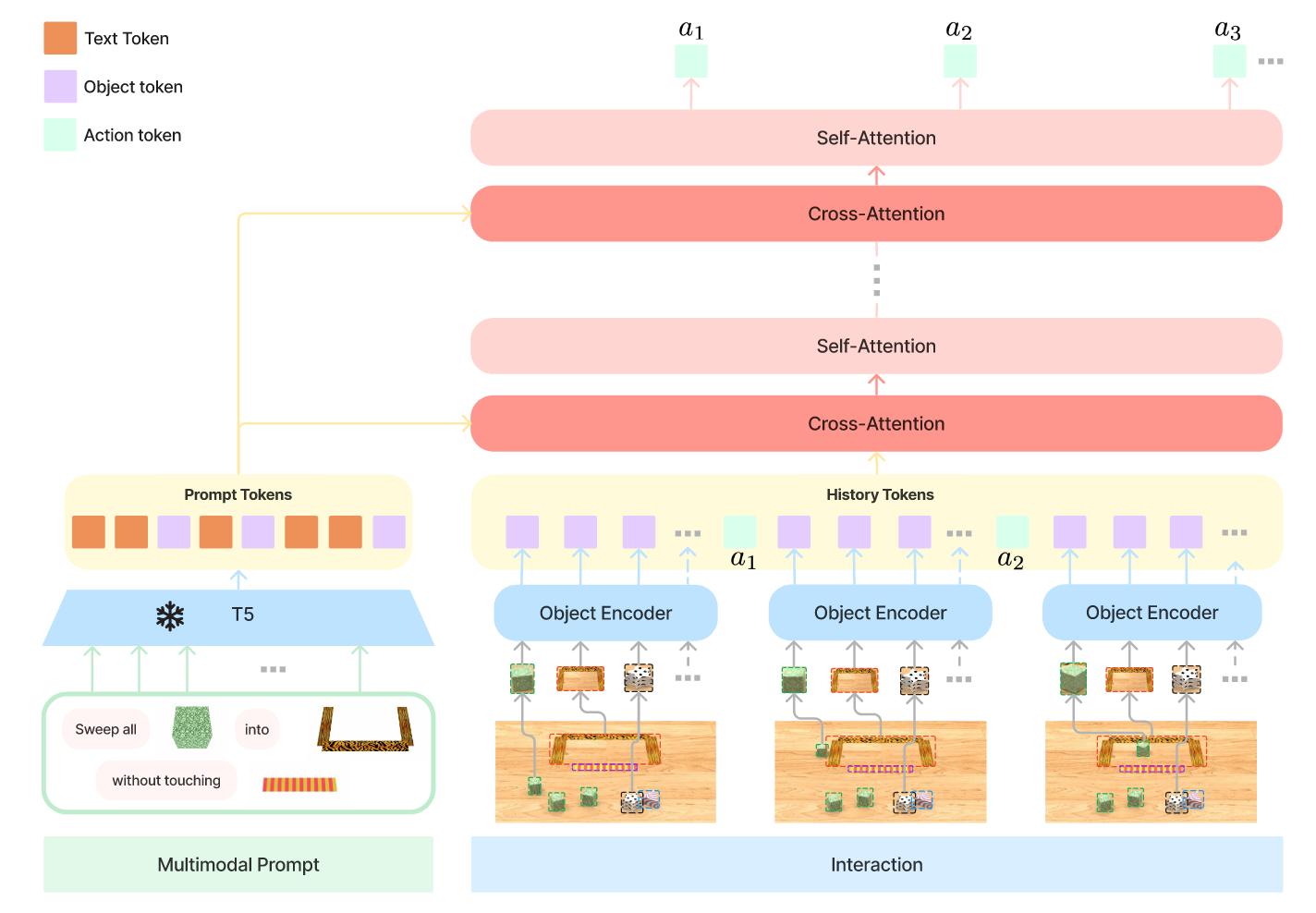
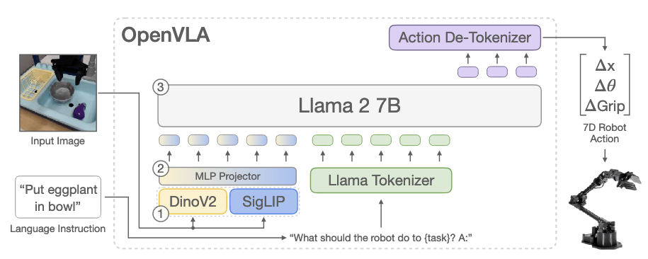
Breck, E., Cai, S., Nielsen, E., Salib, M., & Sculley, D. (2016). What’s your ML test score? A rubric for ML production systems. NIPS Workshop on Reliable Machine Learning in the Wild.
Octo is a transformer-based policy with modular tokenizers (language via T5, images via CNN patches), blockwise masking, and readout tokens, trained on 800k multi-robot trajectories.
Actions are generated through a diffusion head that produces continuous, multimodal, chunked predictions, enabling precise control and broad generalization.
It achieves state-of-the-art zero-shot performance across 7 robots and allows efficient finetuning to new sensors and action spaces, while being fully open-source.
Category
Simple Analogy
Actual Tokenization
Language
[Sentence]
[l₁, l₂, l₃, …] → multiple tokens from a tokenized sentence
Goal Image
[Goal]
[g₁, g₂, g₃, …] → image split into patches
Observation (time t)
[Observation]
[oₜ¹, oₜ², oₜ³, …] → camera frames/sensors tokenized into patches
Readout Token
[ ] (empty slot)
[TR,t] → one per timestep, reserved for predicting actions
Time t-1: [l][g][o_{t-1}][TR,t-1]
Time t: [l][g][o_t][TR,t]
Time t+1: [l][g][o_{t+1}][TR,t+1]
[TR,t-1], [TR,t], [TR,t+1] ──► Diffusion head ──► [a_t, a_{t+1}, …]
GRPs aim for low-level visuomotor control across tasks, environments, and robotic systems.
Existing models often have restricted inputs (e.g., a single camera), lack efficient finetuning to new domains, and importantly, largest models are not publicly available.
Octo = modular, efficient, open-source GRP:
A transformer + diffusion policy trained on large-scale multi-robot data that adapts quickly with little in-domain data to new sensors and action spaces, enabling broad generalization.
Mees, O., Ghosh, D., Pertsch, K., Black, K., Walke, H. R., Dasari, S., Hejna, J., Kreiman, T., Xu, C., & Luo, J. (2024). Octo: An open-source generalist robot policy. First Workshop on Vision-Language Models for Navigation and Manipulation at ICRA 2024.
Inductive learning (귀납적 학습): learning a general function or rule (possibly incorrect) from specific input-output pairs
Bottom to top
Specific to general
Deductive learning (연역적 학습): going from a general rule to a new specific rule that is logically entailed, but is useful because it allows more efficient processing
to predict a continuous value as the output for a given input
weather temperature: solar radiation, wind direction and speed, geographic location..
how to predict the output value of a new data instance on the basis of observed features from the existing data (historical examples) in the problem domain.
Elements
Collection of existing or historical data samples which are represented by a set of attributes or independent variables
The output values of the existing data samples
the output variable or attribute must be continuous
Regressor: a function describes the relationship between the attributes of a data sample and the output.
takes the values of attributes of a data sample and predicts the output value of this given data sample.
Predict the fuel price using the Brent crude oil price, financial performance of the oil related companies (cash flow, projects lined up, etc.) and/or geopolitical risks (OPEC announcements, government sanctions, etc.)
Predict the house price of a suburb from the suburb's profile
Predict the blood pressure of a patient based on the patient's health profile
Predict the electricity price using temperature, demand and time.
to predict discrete or categorical value as the output for a given input
Pass or Failed given learning outcomes, student ID, prior learning, attitude, commitment and attendance.
how to put a new data instance into one of predefined categories or classes on the basis of observed features from the existing data in the problem domain.
Elements
Collection of existing or historical data samples with class labels
Predefined categories or classes
Adequate samples in each category or class in the existing or historical data.
the fundamental quantity in information theory. It is a measure of the uncertainty of a random variable.
the fundamental quantity in information theory. It is a measure of the uncertainty of a random variable
A more homogeneous node with a clear majority class has low impurity and low entropy, while a more mixed distribution of classes has high impurity and high entropy.
The information gain from the attribute test on (split on A) is the expected reduction in entropy.
Information gain computes the difference between entropy before the split and average entropy after the split of the dataset based on given attribute values
combines multiple weak decision tree models to create a stronger learning model.
two types of randomness are introduced to ensure that the individual decision trees are diverse and less prone to overfitting.
Random sampling of the input data
Bootstraping:
involves sampling with replacement 복원추출 (meaning that some instances appearing multiple times and others not appearing) from the original dataset, creating a new dataset.
each decision tree is trained on a slightly different set of data points, reducing the likelihood of overfitting.
Random selection of features at each split
At each split in each decision tree, a random subset of features is considered when determining the best split.
each tree in the ensemble does not rely on the same set of features for making decisions, resulting in a more diverse set of trees.
By considering only a subset of features at each split, the model is less likely to be influenced by a small number of dominant features, leading to a more balanced and accurate prediction.
구분
데이터 무작위성 (Bootstrapping)
속성 무작위성 (Feature Subset Selection)
적용 위치
트리 훈련 데이터 선택 단계
트리의 각 분할(split) 단계
방법
원본 데이터셋에서 복원 추출(with replacement)로 샘플링하여 새로운 학습용 부분집합 생성
전체 속성 중 무작위로 일부 속성만 선택 후, 그 속성들로만 분할 기준 탐색
특징
- 각 나무가 다른 데이터 포인트로 학습됨 - 일부 샘플은 여러 번 등장, 일부는 제외될 수 있음
aggregating the predictions of all individual decision trees in the forest.
Majority voting: For classification, Count the number of times each class is predicted by the individual decision trees. The class with the highest count is considered as the final prediction.
Averaging: For regression, Calculate the mean of the predictions made by the individual decision trees. The mean value is considered as the final prediction.
a learning technique that finds a linear relationship between input variables and the target variable based on a fundamental assumption that there is a linear relationship between input variables and the target variable
e.g. the input variables (engine size, weight and car age) ➡️ target variable (car fuel efficiency)
assumption that there is a linear relationship
A linear regression technique learns a set of coefficients to estimate the linear relationship between x and y, denoted as hw, which can be represented by the following equation.
h_w(x)=w0+w1x1+...+wnxn=∑i=0nwixi
w is a weight vector
y^=∑i=0nwixi
linear regression model is an approximate function between the input variables and the target variable, there will be an error between the output of the model and the actual output value for a data sample
This error can be represented by a loss function, which calculates the mean square error
to find the best linear relationship hwthat best fits the training data of m data samples.
makes the loss to be minimised.
to find the best weight vector w∗, such that for a given training dataset of m data samples.
w∗=argminwLoss(hw)
gradient descent: continuously resamples the gradient of the weight coefficients in the opposite direction depending on the weight w.
Until the loss function Loss(hw) reaches the global minimum
to change the individual components of w a little bit in the direction that minimises Loss(hw), and to do this many times.
wi←wi+α∑j=1mxj,i(yj−hw(xj))
α: the step size, the learning rate
Training model: the process of iteratively updating weights with a learning rate to minimise loss, where the final weight vector defines the model used for predicting new data.
use regularisation on a multivariate linear function to avoid overfitting.
Batch gradient descent: consider the entire training dataset (X,y) at once.
w0←w0+α∑j=1m(yj−(w0+w1xj))
w1←w1+α(∑j=1m(yj−(w0+w1xj))⋅xj)
Stochastic gradient descent (SGD): consider only a single training data sample (xj,yj) at a time.
w0←w0+α(yj−(w0+w1xj))
w1←w1+α((yj−(w0+w1xj))⋅xj)
can be used in an online setting, where new data is coming one at a time, or offline, where we cycle through the same data as many times as is necessary, taking a step after considering each single example.
With a fixed learning rate α, the stochastic version does not guarantee convergence.
often faster than batch gradient descent.
With a schedule of decreasing learning rates (SA), the stochastic version does guarantee convergence.
These update rules are derived as the next weight update equations by taking the partial derivatives of the loss function with respect to w0 and w1.
an extension of linear regression in such a way that the output of a linear regression model goes through a logistic function
y(x)=1+e−x1
The output value of this logistic function is between 0 and 1.
0 is for certainly being labeled "0" and 1 is for certainly being labeled "1", and a value between 0 and 1 represents the probability of being labeled "1"
a logistic regression model: a linear regression model + a logistic function
Conceptually trivial: Given a set of N examples and a query xq, iterate through the examples, measure the distance to xq from each one, and keep the best k.
NN(k,xq)'s time complexity is O(N), N is the number of examples in the training dataset.
Use a k-dimensional tree: a balanced binary tree with an arbitrary number of dimensions.
Time complexity can be improved to O(logN)
appropriate only when there are many more examples than dimensions
It works well with up to 10 dimensions with thousands of examples.
Use a Hash table with a locality-sensitive hash (LSH)
the largest possible distance to example points, helping to improve generalization
SVMs create a linear separating hyperplane
kernel trick: to embed the data into a higher-dimensional space
Often data that are not linearly separable in the original input space are easily separable in a higher-dimensional space
In general (excepted some special cases) if we have N data points then they will always be separable in spaces of N dimensions or more
SVMs are a nonparametric method
retain training examples and potentially need to store them all
In practice, they often end up retaining only a small fraction of examples
have the flexibility to represent complex functions, but they are resistant to overfitting
not usually expect to find a linear separator in the input space x, but we can find linear separators in the high-dimensional feature space F(x) simply by replacing (xjxk) in
argmaxα∑jαj−21∑j,kαjαkyjyk(xj⋅xk)
with K(xj,xk)=F(xj)⋅F(xk)
F(xj)⋅F(xk) can often be computed without first computing F for each point.
In a higher dimensional feature space, which is created by transformation F(x), if we can express K(xj⋅xk)=F(xj)⋅F(xk), the kernel function K(xj⋅xk) can be applied to pairs of input data to evaluate dot product in some corresponding feature space.
kernel trick is to plug a kernel function K(xj⋅xk) into the dual optimisation problem to replace (xj⋅xk)
Optimal linear separators can be found efficiently in feature spaces with billions of (or, in some cases, infinitely many) dimensions.
we can learn in the higher-dimensional space, but we compute only kernel functions rather than the full list of features for each data point.
Symbol understanding (e.g., “move apple to 3 / heart / star”).
Reasoning (visual matching, simple math like “sum of two plus one”, multilingual commands).
Human recognition (e.g., “person with glasses”); none of these were present as low-level actions in robot data.
Chain-of-thought (CoT) variant adds a Plan step before actions → supports multi-stage semantic reasoning (e.g., pick a rock as an improvised hammer; pick an energy drink for a tired person).
Zitkovich, B., Yu, T., Xu, S., Xu, P., Xiao, T., Xia, F., Wu, J., Wohlhart, P., Welker, S., Wahid, A., Vuong, Q., Vanhoucke, V., Tran, H., Soricut, R., Singh, A., Singh, J., Sermanet, P., Sanketi, P. R., Salazar, G., Ryoo, M. S., Reymann, K., Rao, K., Pertsch, K., Mordatch, I., Michalewski, H., Lu, Y., Levine, S., Lee, L., Lee, T.-W. E., Leal, I., Kuang, Y., Kalashnikov, D., Julian, R., Joshi, N. J., Irpan, A., Ichter, B., Hsu, J., Herzog, A., Hausman, K., Gopalakrishnan, K., Fu, C., Florence, P., Finn, C., Dubey, K. A., Driess, D., Ding, T., Choromanski, K. M., Chen, X., Chebotar, Y., Carbajal, J., Brown, N., Brohan, A., Arenas, M. G., & Han, K. (2023). RT-2: Vision-Language-Action Models Transfer Web Knowledge to Robotic Control Proceedings of The 7th Conference on Robot Learning, Proceedings of Machine Learning Research. https://proceedings.mlr.press/v229/zitkovich23a.html
ViT (e.g., ViT-4B, ViT-22B) extracts image embeddings.
OSRT builds object-centric slot representations.
These are injected into the LLM embedding space (PaLM variants: 8B, 62B, 540B) for high-level abstraction and planning, with execution delegated to low-level policies (e.g., RT-1).
Build embodied language models by injecting continuous sensor inputs (images, states, other modalities) directly into a pretrained LLM’s embedding space, linking words ↔ percepts.
Inputs are multimodal sentences that interleave text tokens with encoded visual/state tokens; outputs are text (answers or high-level plans).
Start from a decoder-only, autoregressive LLM (PaLM) and condition on a prefix that mixes text and encoder-produced vectors.
Provide multiple encoder options:
State vectors (simplest).
ViT features with a learned projector ψ to match LLM embedding dimensionality.
Object-centric, 3D-aware OSRT (neural scene representations). Supports entity-label tokens (<obj j>) so the model can refer to specific objects in generated plans.
For planning/control, PaLM-E emits textual subgoals/skills drawn from a small skill vocabulary; a separate low-level policy executes them.
The system runs closed-loop: execute → observe → (re)plan; PaLM-E acts as a high-level policy sequencing low-level skills.
Why not text-only LLMs or affordance-only grounding?
Prior work that feeds only text to the LLM (and uses external affordance models) is insufficient when spatial layout matters.
PaLM-E instead grounds inside the LLM by injecting continuous observations, enabling direct plan generation while leveraging the LLM’s world knowledge.
Transfer via co-training: One model trained on mixed tasks/embodiments achieves higher performance than task-specialists; "full mixture" yields >2× gains (Fig. 3).
Few-shot/data efficiency: Solves robotics tasks with very few examples (e.g., 10–80 for Language-Table, 320 for TAMP). OSRT further improves data efficiency.
Mobile manipulation: End-to-end embodied planning works in real kitchens, robust to disturbances; PaLM-E beats PaLI (zero-shot) and QT-OPT/CLIP baselines on affordance/failure detection.
General V+L: The 562B generalist achieves state-of-the-art on OK-VQA and strong VQAv2/COCO without task-specific finetuning.
Language retention & scaling: Freezing LLM preserves language ability but can struggle on some robotics tasks; unfrozen + scale up significantly reduces catastrophic forgetting.
Emergent behaviors: Multimodal chain-of-thought and multi-image reasoning emerge in PaLM-E-562B, despite training on single-image prompts.
Driess, D., Xia, F., Sajjadi, M. S. M., Lynch, C., Chowdhery, A., Ichter, B., Wahid, A., Tompson, J., Vuong, Q., Yu, T., Huang, W., Chebotar, Y., Sermanet, P., Duckworth, D., Levine, S., Vanhoucke, V., Hausman, K., Toussaint, M., Greff, K., Zeng, A., Mordatch, I., & Florence, P. (2023). PaLM-E: An Embodied Multimodal Language Model Proceedings of the 40th International Conference on Machine Learning, Proceedings of Machine Learning Research. https://proceedings.mlr.press/v202/driess23a.html