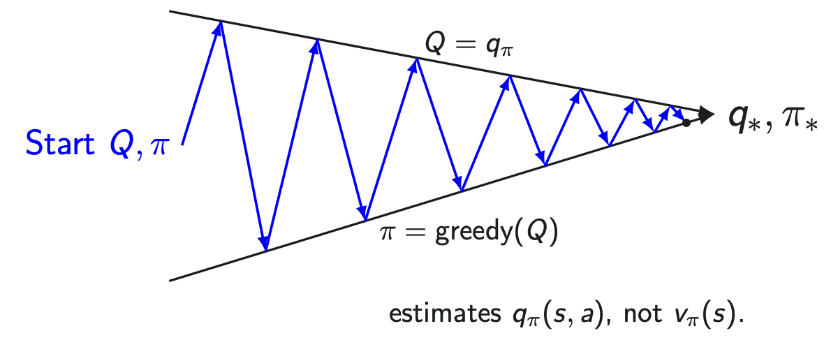
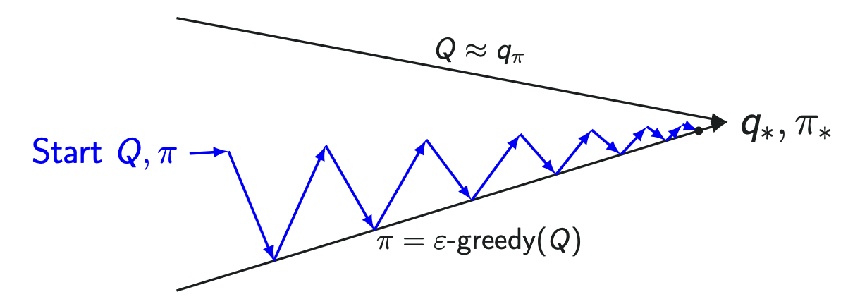
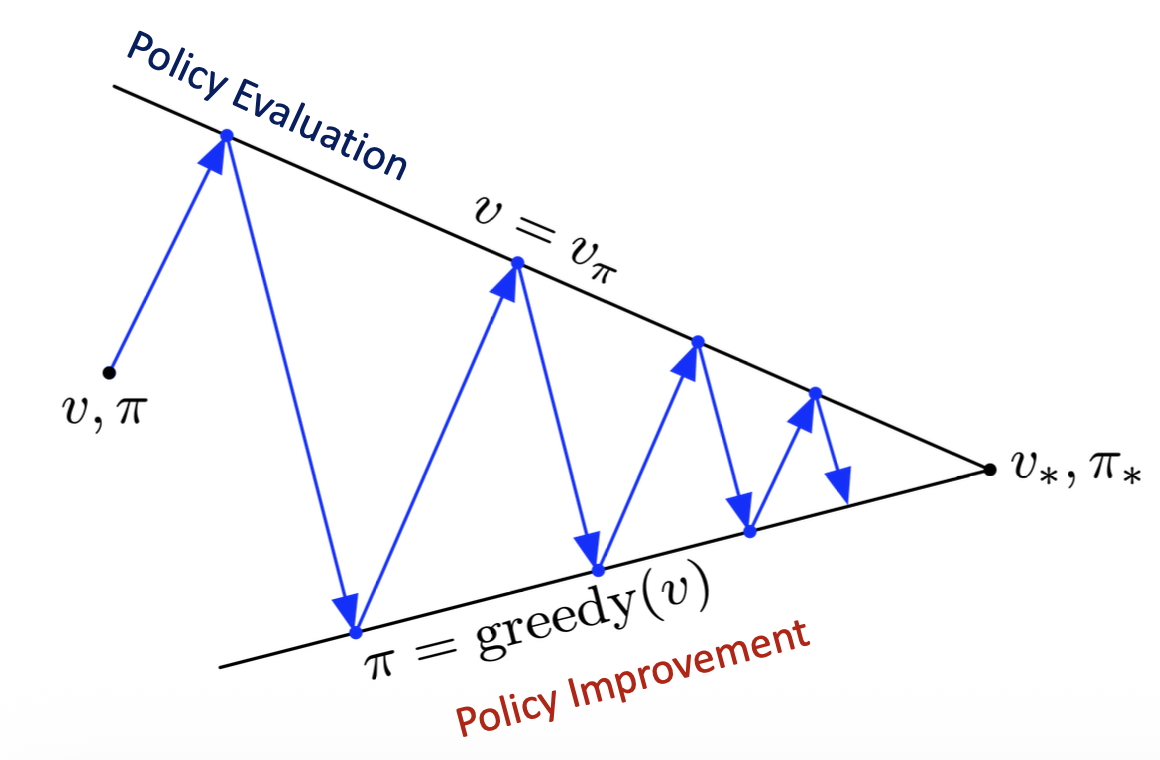
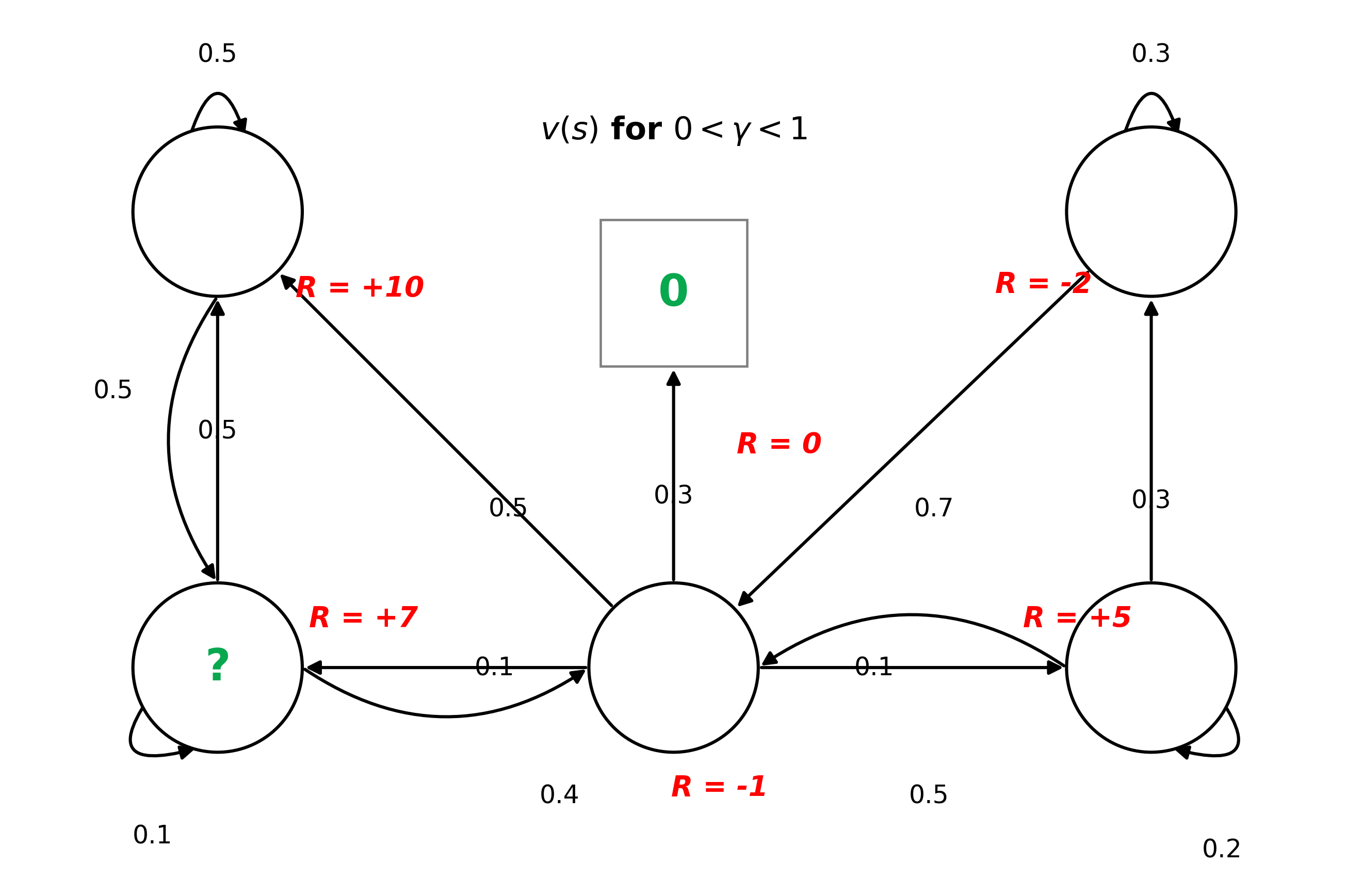
Given a policy πθ(a∣s) with parameters θ, the goal is to find the best θ.
J1(θ)=vπθ(S1)
In an episodic task (with an end state), J1(θ) is for that particular start state and measures how much expected return we can get.
S1 is the start state.
J(θ) is the measure of the quality of the policy or the objective function to optimize.
JavV(θ)=s∑μπθ(s)vπθ(s)
In continuing environments (doesn't have an end state), consider the states and take the average value weighted by how often the agent visits each state.
μπθ(s) is how often the agent is visiting that particular state s.
JavR(θ)=s∑μπθ(s)a∑πθ(a∣s)r∑p(r∣s,a)r
Use the average reward per time step.
Small batches can be used to estimate this average reward during training.
Input: a differentiable policy parameterization π(a∣s,θ)Algorithm parameter: step size α>0Initialize policy parameter θ∈Rd′ (e.g., to 0)Loop forever (for each episode):Generate an episode S0,A0,R1,…,ST−1,AT−1,RT, following π(⋅∣⋅,θ)Loop for each step of the episode t=0,1,…,T−1:G←∑k=t+1Tγk−t−1Rk(Gt)θ←θ+αγtG∇lnπ(At∣St,θ)
Input: a differentiable policy parameterization π(a∣s,θ)Input: a differentiable state-value function parameterization v^(s,w)Parameters: step sizes αθ>0,αw>0Initialize policy parameter θ∈Rd′ and state-value weights w∈Rd (e.g., to 0)Loop forever (for each episode):Initialize S (first state of episode)I←1Loop while S is not terminal (for each time step):A∼π(⋅∣S,θ)Take action A,observe S′,Rδ←R+γv^(S′,w)−v^(S,w)(if S′ is terminal, then v^(S′,w)≐0)w←w+αwδ∇v^(S,w)θ←θ+αθIδ∇lnπ(A∣S,θ)I←γIS←S′
It quantifies how much one probability distribution differs from another probability distribution.
∣∣ indicates divergence or P's divergence from Q.
DKL(P∣∣Q)=∑x∈XP(x)logQ(x)P(x)
Given two probability distributions P and Q over a discrete random variable X, the KL divergence is the expected value under P of the log ratio between P and Q.
Multiplying by P(x) gives more weight to events that occur frequently under P.
P large, Q small → large divergence
P small, Q large → effect is smaller
e.g. πold(a1∣s)=0.8 and πold(a2∣s)=0.2, while πnew(a1∣s)=0.1 and πnew(a2∣s)=0.9
The policy changed drastically in one update step.
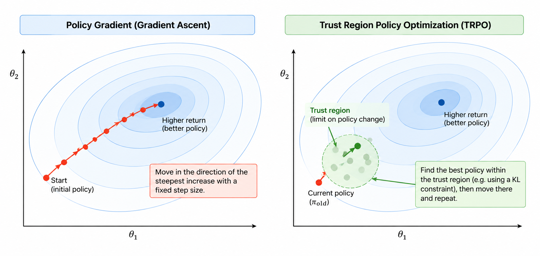
TRPO prevents this by enforcing DKL(πold∥πnew)≤δ.
rt(θ)=πθold(at∣st)πθ(at∣st) is the ratio of the new policy to the old policy.
A^t=Q(st,at)−V(st) is the advantage function.
ϵ is a hyperparameter, usually 0.1 or 0.2.
If ϵ=0.2, the clipping range is [0.8,1.2].
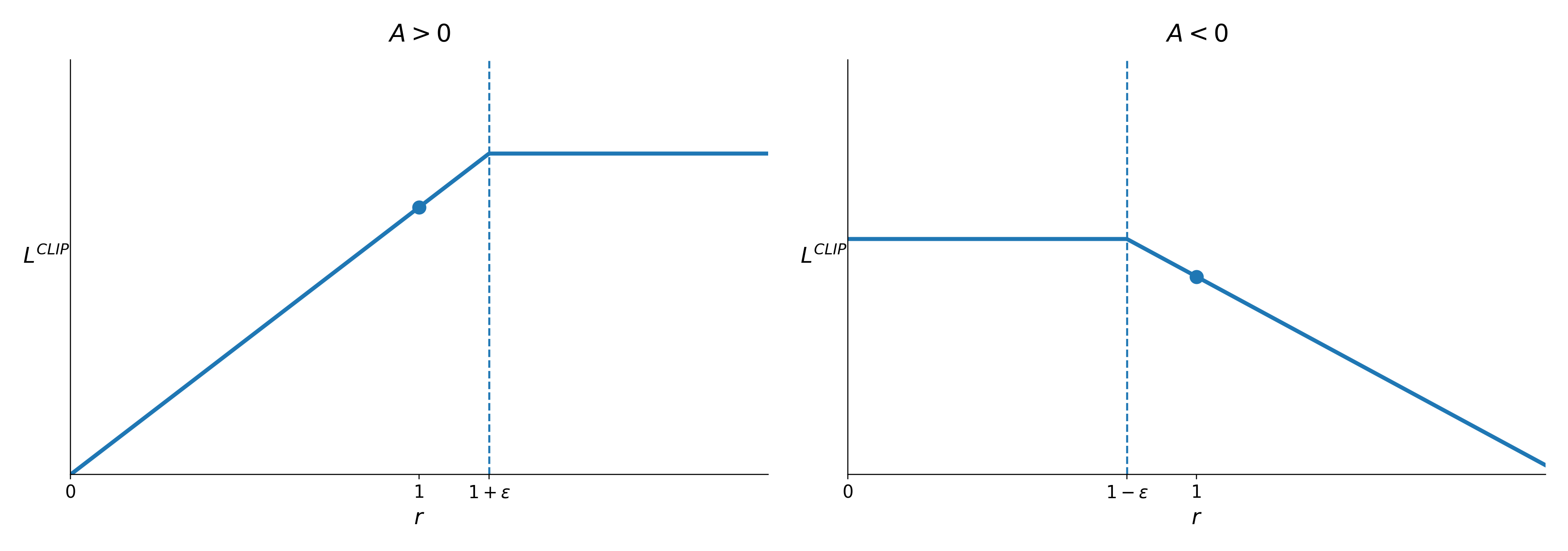
For A^t>0, PPO removes the benefit of increasing rt above 1+ϵ.
For A^t<0, PPO removes the benefit of decreasing rt below 1−ϵ.
The policy ratio itself is not strictly forced to remain inside the clipping range.
Instead, clipping removes the incentive for excessively large beneficial policy updates.
Algorithm: PPO with Clipped ObjectiveInput: θ0,ϵfor k=0,1,2,… doCollect set of partial trajectories Dk on policy πk=π(θk)Estimate advantages A^tπk using any advantage estimation algorithmCompute policy updateθk+1=argmaxθLθkCLIP(θ)by taking K steps of minibatch SGD (via Adam), whereLθkCLIP(θ)=Eτ∼πk[∑t=0Tmin(rt(θ)A^tπk,clip(rt(θ),1−ϵ,1+ϵ)A^tπk)]
θ0: Initial policy parameters.
ϵ: Clipping threshold.
A^tπk: Aπ(s,a)=Qπ(s,a)−Vπ(s), where at∼π(at∣st),st+1∼P(st+1∣st,at), for t≥0.
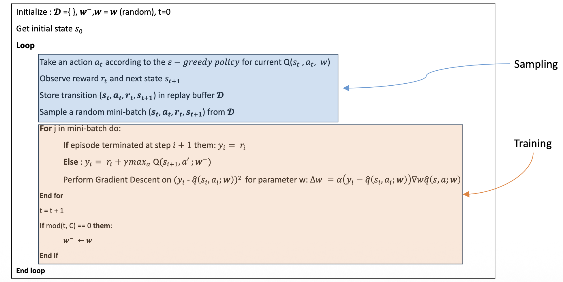
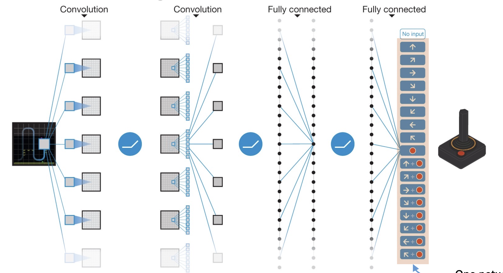
DQN stores past transitions (s,a,r,s′) in a replay buffer and randomly samples them for training, which reduces correlation between consecutive samples and improves training stability.
Sample (s,a,r,s′) from D
Compute the target value of the samples s:(r+γmaxa′q^(s′,a′,w))
Use SGD to update the network weight: Δw=α(r+γmaxa′q^(s′,a′,w)−q^(s,a,w))∇wq^(s,a,w)
Initialize w=0,k=1Loop:Sample k-th episode (sk1,ak1,rk1,...,SkLk) using policy πFor t=1,...Lk:if First Visit to (s) in episode k,thenGt(s)=j=t∑Lkγk,jWeight update: w←w−α(Gt−v^(s,w))x(s)k=k+1
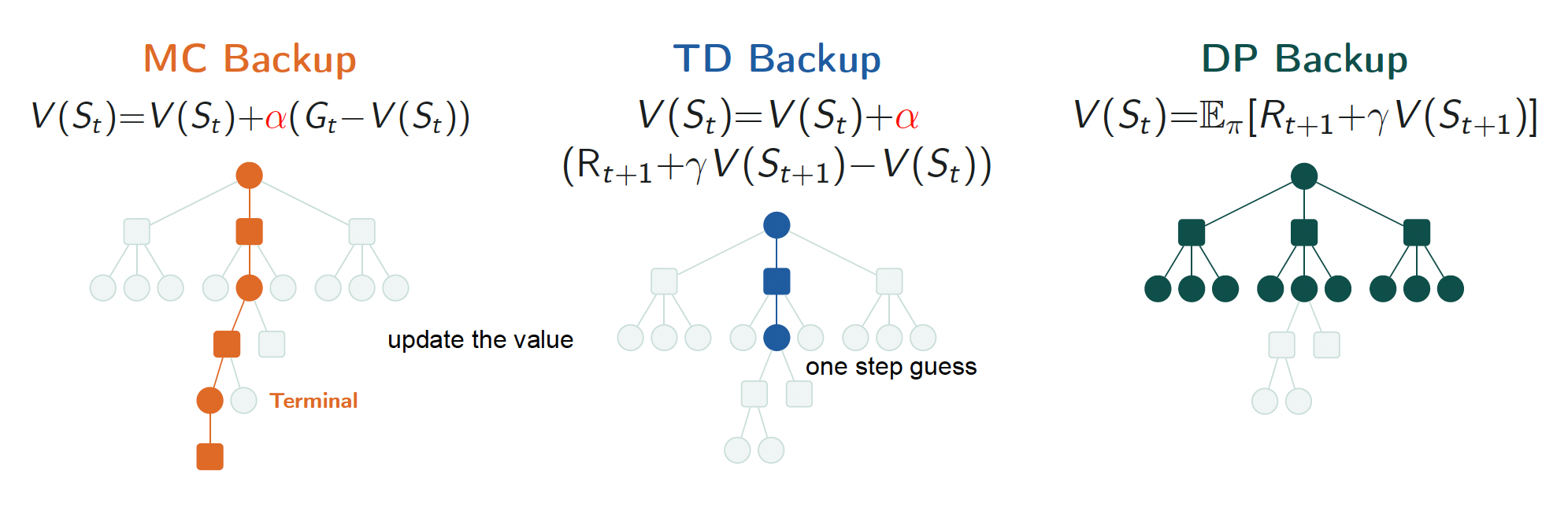
Loop for each episode:InitializeSLoop for each step of the episode:A←action given by policyπTake actionA,observeR,S′V(S)←V(S)+α[R+γV(S′)−V(S)]S←S′UntilS is terminal
No need to wait until the end of the episode to update the value function.
Loop for each episode:InitializeSChooseAt from St using policy π derived from QLoop for each step of the episode:Take actionAt+1,observeRt+1,St+1Q(St,At)←Q(St,At)+α[Rt+1+γQ(St+1,At+1)−Q(St,At)]St←St+1At←At+1UntilS is terminal
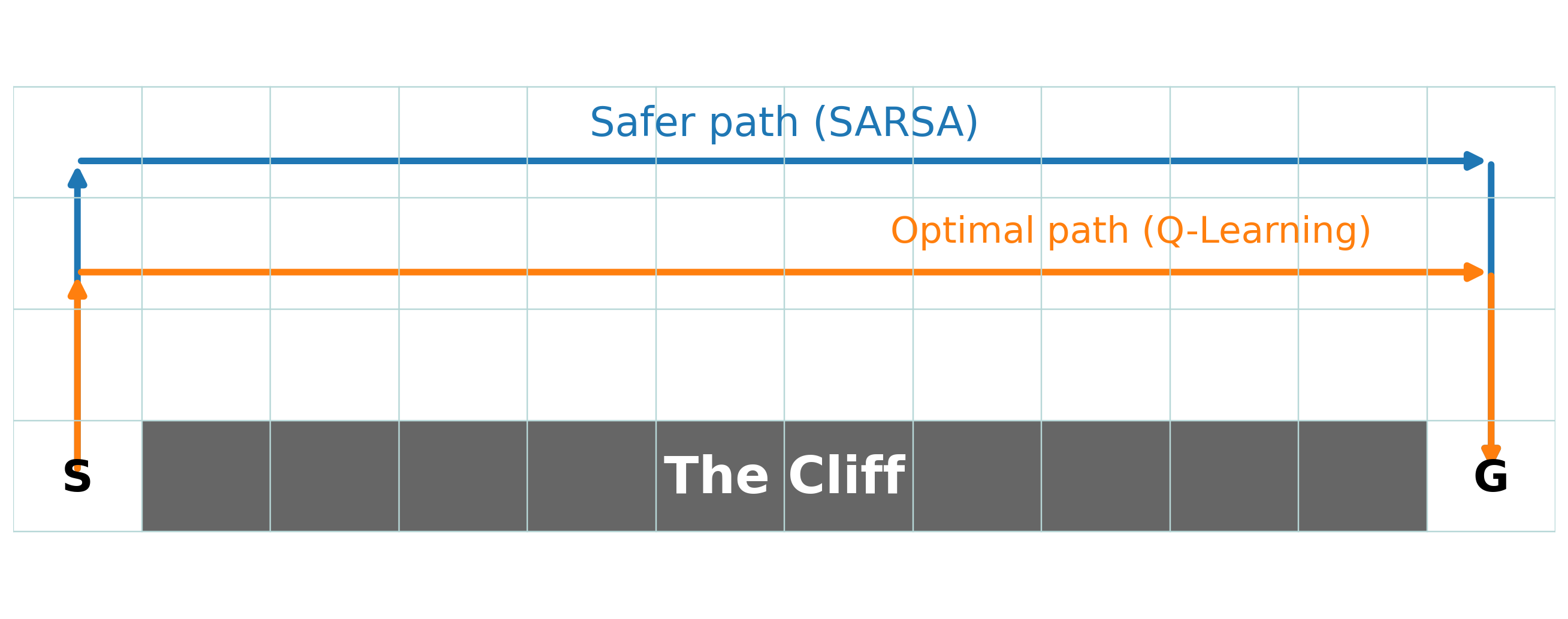
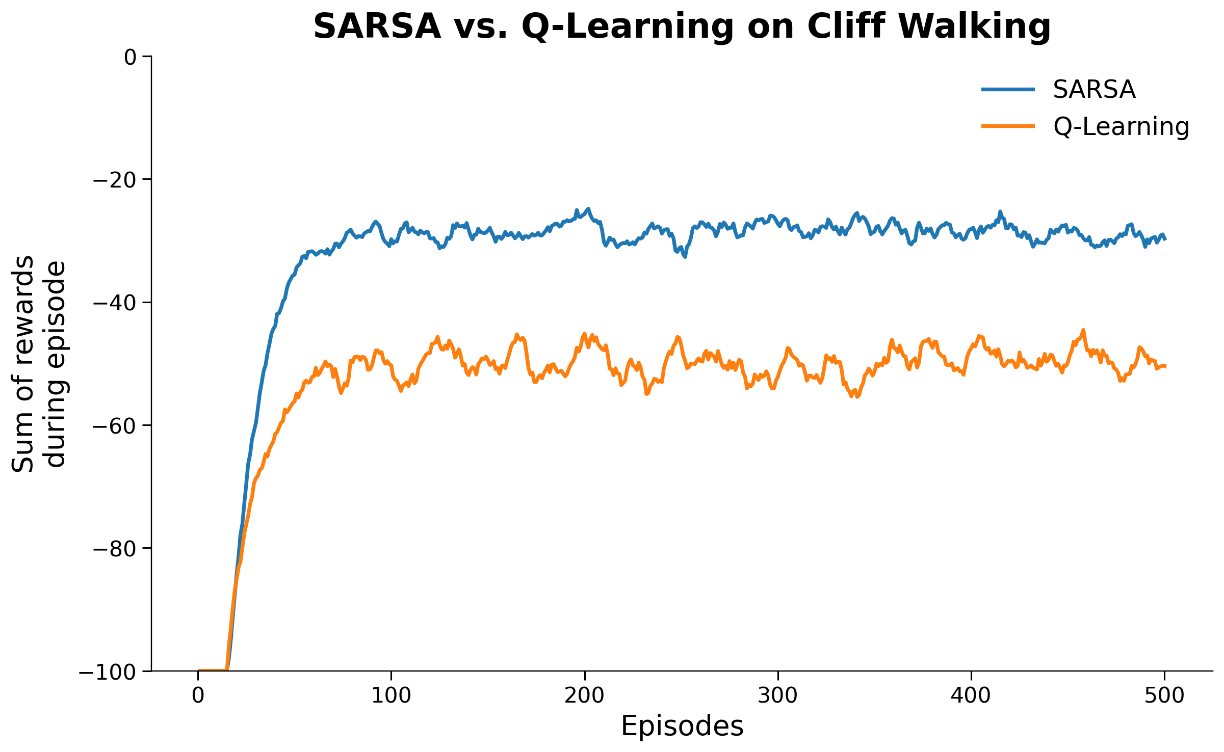
As SARSA learns, each episode is completed faster.
As the Q-values improve, the agent learns better actions for each state and reaches the goal using fewer steps.
Loop for each episode:InitializeSLoop for each step of the episode:At fromSt using policy π derived from QTake actionAt+1,observeRt+1,St+1Q(St,At)←Q(St,At)+α[Rt+1+γamaxQ(St+1,a)−Q(St,At)]St←St+1UntilS is terminal
Model-Free Learning: Operates without prior knowledge of transition dynamics P or reward function R.
Learning from Complete Episodes: Learns state-value functions vπ exclusively from full trajectories under policy π. Only works for episodic tasks where termination at step T is guaranteed.
No Bootstrapping: Does not update estimates using other value estimates v(s′); instead, updates rely solely on actual empirical returns observed at the end of the episode.
Empirical Mean Returns: The value of state s is estimated by the sample average of all observed returns starting from s:
Discount Factor (γ=1): For episodic tasks with terminal-only rewards (such as Blackjack), setting γ=1 is standard practice because the episode length is finite.
Every-Visit MC treats every single occurrence of state s within an episode as a valid data sample, accumulating its corresponding return into the empirical mean.
Algorithmic Flow:
Initialize counters N(s)←0 and accumulate returns: G(s)←0∀s∈S
Sample a complete episode i={Si,0,Ai,1,Ri,2,…,Si,Ti} generated under policy π
Compute return Gi,t=∑k=t+1Tiγk−t−1Ri,k from step t to termination.
For each time step t where state s appears in episode i:
N(s)←N(s)+1 (Increment counter for total visits)
G(s)←G(s)+Gi,t (Increment total return)
V(s)←N(s)G(s) (Update the value by mean return)
AR1=1BR2=2AR3=1CR4=1terminal
State s
N(s)
G(s)
V(s)=N(s)G(s)
A
2
9+6=15
7.50
B
1
8
8.00
C
1
5
5.00
Dimension
First-Visit MC
Every-Visit MC
Returns used per episode
Only the first occurrence
Every occurrence
Sample independence
Independent across episodes (i.i.d.)
Correlated within an episode (mitigated by sampling)
Updates the value function V(s) incrementally after each trajectory without requiring memory to store individual past returns.
Algorithmic Flow:
Initialize N(s)←0 and V(s)←0 for all s∈S.
Episode sampling: Execute episode i under policy π and compute returns Gi,t=∑k=t+1Tiγk−t−1Rk.
Incremental update: For each visited state s at time step t:
N(s)←N(s)+1 (Increment counter for total visits)
V(s)←V(s)+α(Gi,t−V(s)) (Update the value by mean return)
Where Gi,t−V(s) represents the temporal difference (TD) error between the sampled return target and the current estimate.
Choice step size α
α=N(s)1: Replicates the exact empirical sample-average of Every-Visit MC where all observed samples receive equal weight.
α=constant: Implements an exponential recency-weighted running average that decays outdated experience, making it suited for non-stationary environments where MDP dynamics change over time.
Cons:
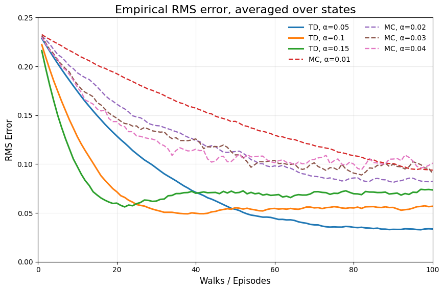
Requires a significant number of episodes to converge to the true value function.
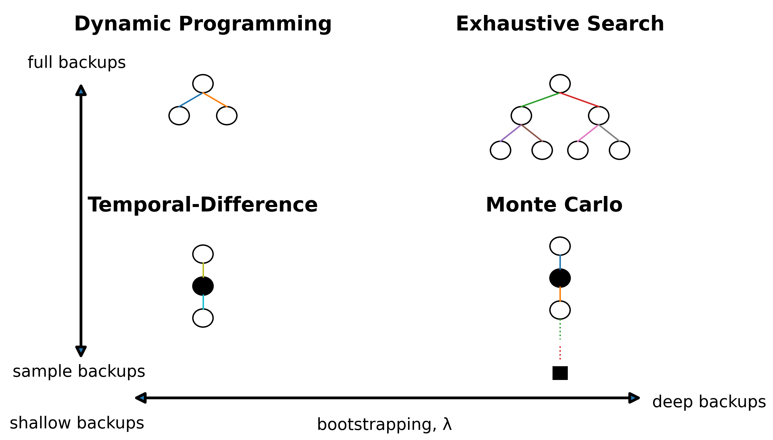
A foundational and efficient framework widely used for solving MDPs.
Mathematically guaranteed to converge to an optimal policy in polynomial time in terms of the number of states and actions.
Exponentially faster than exhaustive direct search across the policy space (∣A∣∣S∣).
Limitations:
Can become computationally impractical for extremely large or complex environments.
Curse of Dimensionality: As the number of state variables (dimensions) increases, the total state space size (∣S∣) expands exponentially, leading to severe computational and memory bottlenecks.
Comparison with Synchronous Methods: Standard DP methods sweep through the entire state space systematically in every iteration. Asynchronous DP backs up individual states independently in arbitrary order.
In-place Value Updates: Directly overwrites values in a single memory array, allowing immediate propagation of newly updated state values to subsequent calculations.
Computational Gain & Convergence:
Significantly reduces computation by avoiding exhaustive full-state sweeps.
Guaranteed to converge to the optimal value function v∗, provided that all states continue to be selected and updated indefinitely.
Interaction-Driven Online Updates: Solves sub-problems on-the-fly by focusing updates specifically on states that are directly relevant to the agent's current trajectory.
Target Applications: Large-scale environments where full state-space iteration is intractable (e.g., robotics, autonomous control systems, game AI).
Core Characteristics:
Online Decision Making: Makes and refines decisions while operating directly in the environment.
Lazy Evaluation: Computes values only for visited or critical state subsets rather than unvisited distant states.
Adaptive Exploration: Guides search toward high-reward trajectories through active interaction.
Approximate MDP Solution: Yields near-optimal policies for relevant regions without solving the global MDP.
Motivation: Addresses the curse of dimensionality where tabular representation of states and exact value computation become computationally infeasible.
Function Approximation Methods: Parameterizes and estimates the value function using scalable statistical and machine learning models:
Linear models, deep neural networks, decision trees, and general regression techniques.
Error Management Mechanisms:
Eligibility Traces: Accelerates credit assignment and temporal consistency across multi-step transitions.
Experience Replay: Stores transition tuples in a replay buffer and samples them randomly to break data correlation and stabilize value approximation.
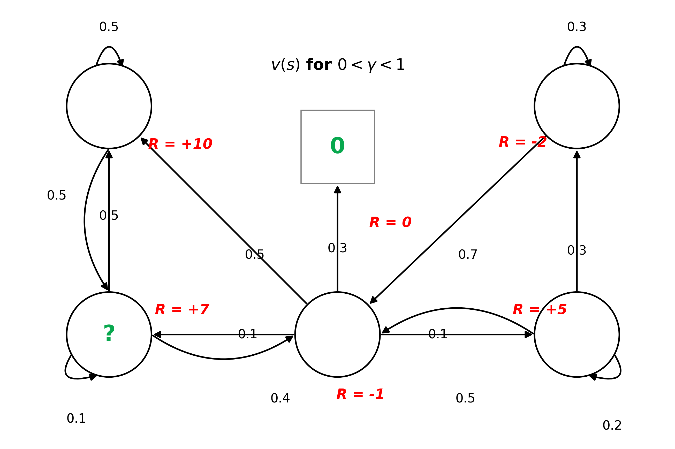
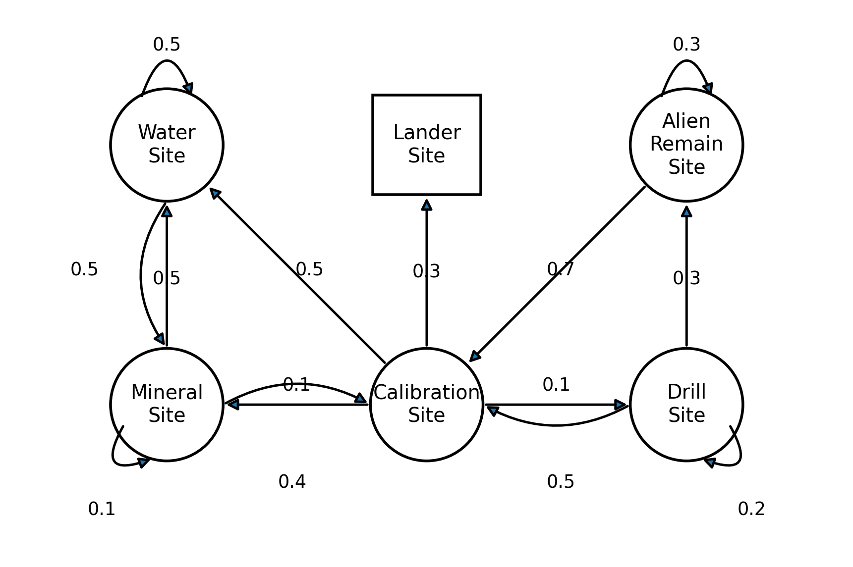
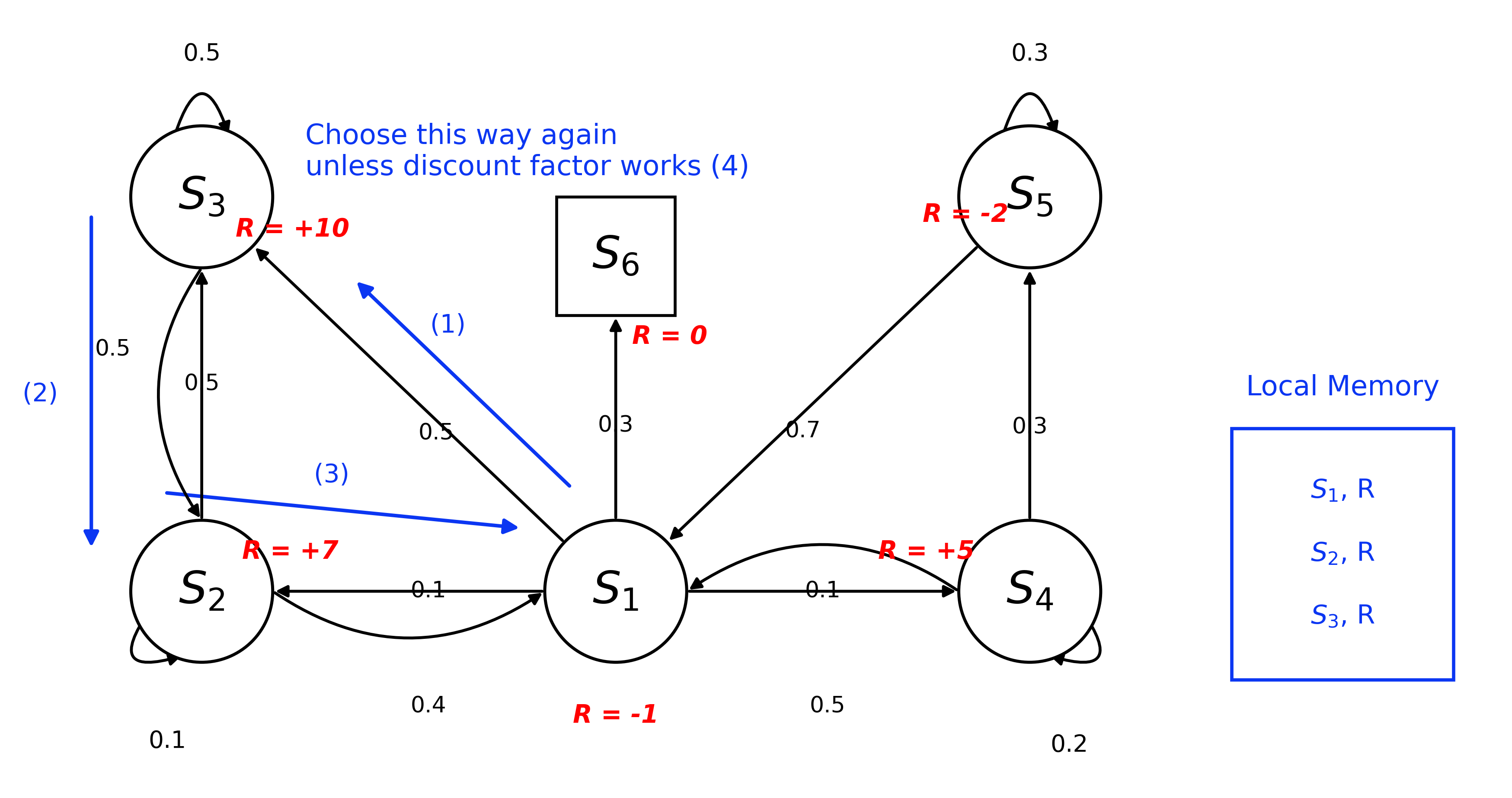
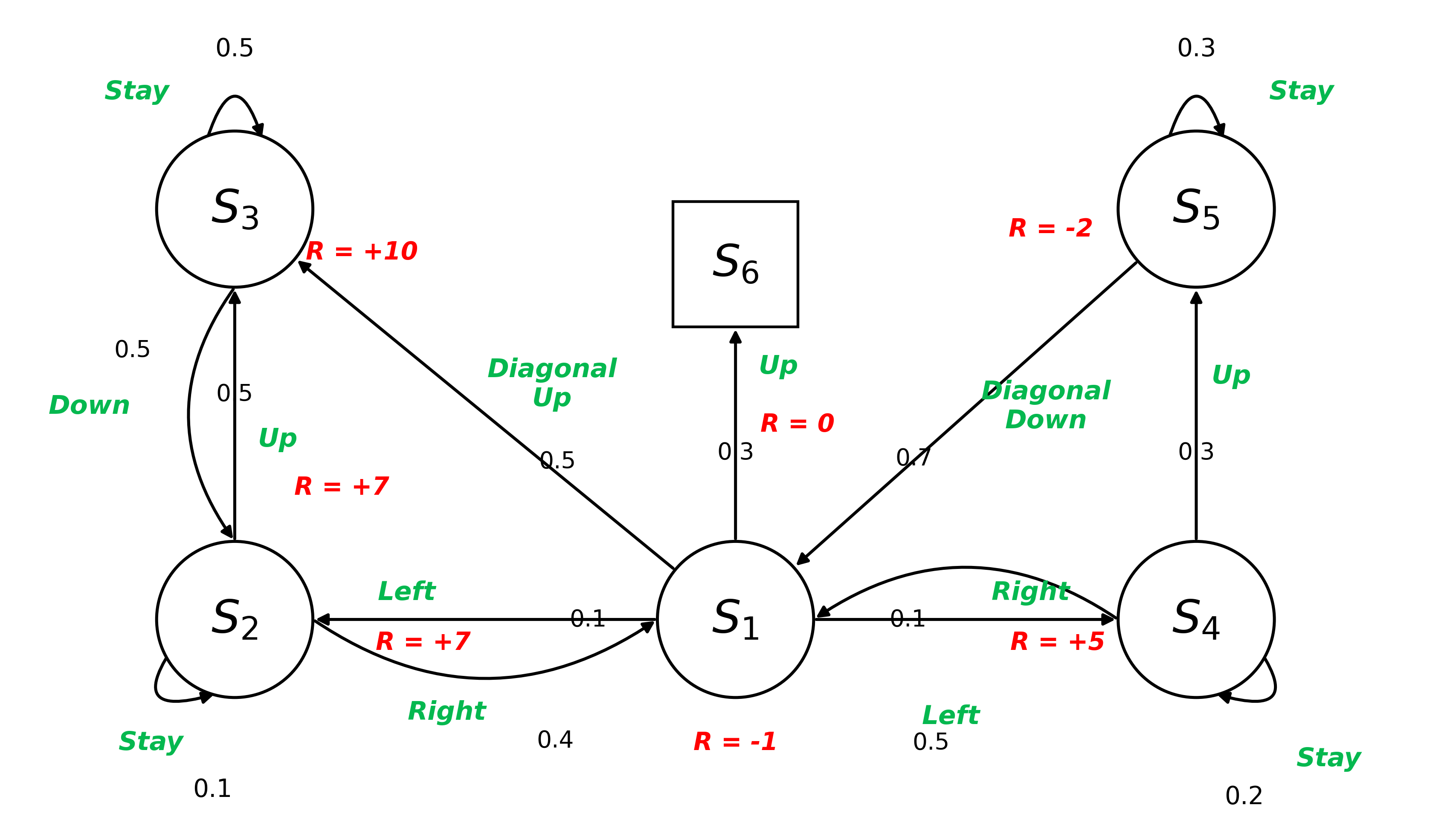
vπ(s)=EπImmediate RewardRt+1+γDiscounted Future Valuevπ(St+1)Starting at state sSt=s
Fundamental concept in RL using a recursive equation to express a way to compute the value of a state based on the values of its successor states.
v(s)=E[Rt+1+γRt+2+γ2Rt+3+…St=s]=ERt+1+γGt+1(Rt+2+γRt+3+…)St=s=E[Rt+1+γGt+1∣St=s]=E[Rt+1+γv(St+1)∣St=s]=Immediate Reward R(s)E[Rt+1∣St=s]+γExpected Next State ValueE[v(St+1)∣St=s]=R(s)+γTransition Dynamicss′∑P(s′∣s)v(s′)(∵E[X+γY]=E[X]+γE[Y])(∵E[g(X)]=x∑P(x)g(x))
V of a particular statev(s1)⋮v(sn)=Immediate RewardR(s1)⋮R(sn)+γTransition MatrixP11⋮Pn1⋯⋱⋯P1n⋮PnnV of future statev(s1)⋮v(sn)
Action-Value of (s,a)qπ(s,a)=Follows policy πEπImmediate RewardRt+1+γDiscounted Next Action-Valueqπ(St+1,At+1)Starting at s taking action aSt=s,At=a
Evaluates the expected return of taking an arbitrary action a in state s, and subsequently following policy π from step t+1 onward.
How good is it to take action a in state s?
qπ(s,a): Value of taking action a in state s under policy π (Q-value).
Eπ: Expectation over the next transition (St+1∼P) and the subsequent action (At+1∼π).
Rt+1: Immediate reward resulting from the state-action pair (s,a).
γqπ(St+1,At+1): Discounted expected value of the successor state-action pair (St+1,At+1).
St=s,At=a: Condition that both the initial state and the initial action are fixed at time t.
vπ(s)=a∈A∑π(a∣s)(Rsa+γs′∈S∑Pss′avπ(s′))
Evaluates state s directly by averaging over all possible action branches (π) and their subsequent environmental transitions (P).
Rsa: Immediate reward resulting from the state-action pair (s,a).
γ∑s′∈SPss′avπ(s′): Discounted expected value of the successor state s′ resulting from the state-action pair (s,a).
Pss′a: Probability of transitioning from state s to state s′ when action a is taken.
S: Set of all possible states.
A: Set of all possible actions.
π(a∣s): Probability of taking action a in state s under policy π.
Evaluates the state-action pair (s,a) by summing immediate reward and the expected value of future action pairs (s′,a′), averaged across transition dynamics P and next-step policy choices π.
Rsa: Immediate reward resulting from the state-action pair (s,a).
γ∑s′∈SPss′a∑a′∈Aπ(a′∣s′)qπ(s′,a′): Discounted expected value of the successor state-action pair (s′,a′) resulting from the state-action pair (s,a).
Pss′a: Probability of transitioning from state s to state s′ when action a is taken.
S: Set of all possible states.
A: Set of all possible actions.
π(a′∣s′): Probability of taking action a′ in state s′ under policy π.
Maximum value function over all policies, or maximum possible reward that can be achieved from state s.
q∗(s,a)=maxπqπ(s,a)
The Optimal Action-Value Function q∗(s,a)
Maximum action-value function over all policies, or given state s and action taken a, what is the maximum reward that can be achieved from there onwards.
Existence of an Optimal Policy: There always exists at least one optimal policy π∗ that is better than or equal to all other policies across all states (π∗≥π,∀π).
Uniqueness of the Optimal State-Value Function: Although multiple distinct optimal policies may exist (e.g., when two different paths yield the exact same maximum expected return), all optimal policies achieve the exact same unique optimal state-value function (vπ∗(s)=v∗(s)).
Uniqueness of the Optimal Action-Value Function: Similarly, all optimal policies achieve the exact same unique optimal action-value function (qπ∗(s,a)=q∗(s,a)).
Once the action a is committed, the outcome is governed by the environment dynamics Pss′a, requiring an expectation (average) over possible successor states s′.
Optimal Value of State sv∗(s)=a∈AmaxImmediate RewardRsa+γExpected Optimal Future Values′∈S∑Pss′av∗(s′)
Bellman Optimality Equation for v∗ (s→a→s′)
Combines the agent's deterministic maximization (maxa) with the environment's stochastic transition (∑s′Pss′a).
It means a structure where the best choice I can make (max) embeds the probabilistic outcomes of the world (∑) in its calculation.
Non-Linear System: Because of the max operator, this system of equations cannot be solved directly via matrix inversion (I−γP)−1
it must be solved iteratively via Dynamic Programming (Value Iteration) or Reinforcement Learning.
Optimal Action-Valueq∗(s,a)=Immediate RewardRsa+γTransition Dynamicss′∈S∑Pss′aOptimal Successor Actiona′∈Amaxq∗(s′,a′)
Bellman Optimality Equation for q∗ ((s,a)→s′→a′)
Action Commitment: The initial state s and action a are fixed, receiving immediate reward Rsa.
Stochastic Transition: The agent transitions to successor state s′ according to the environment's transition probability Pss′a.
Greedy Successor Action (maxa′): Upon landing in state s′, the agent greedily selects the action a′ that yields the maximum possible optimal action-value q∗(s′,a′).
Core Foundation of Q-Learning: This equation directly forms the update target for off-policy algorithms like Q-Learning and DQN
Q(St,At)←Q(St,At)+αOff-policy Target from q∗Rt+1+γamaxQ(St+1,a)−Q(St,At)
Q-Learning (Off-Policy TD Control): Learns optimal action-values q∗ directly from experience tuples (St,At,Rt+1,St+1) by approximating the Bellman Optimality Equation via bootstrapping.
Q(St,At)←Q(St,At)+αOn-policy Target from qπRt+1+γQ(St+1,At+1)−Q(St,At)
SARSA (On-Policy TD Control): Learns action-values qπ for the current policy from experience transitions (St,At,Rt+1,St+1,At+1), steadily improving the policy toward optimality.
Evaluate a given policy π is a prediction problem.
Iterative application of Bellman Expectation backup.
Input:π:Policy to be evaluatedParameters:θ>0:Small threshold determining estimation accuracyγ∈[0,1]:Discount factorInitialize:V(s)∈R,∀s∈SV(terminal)=0Repeat:Δ←0For each s∈S:v←V(s)V(s)←a∈A∑π(a∣s)(Rsa+γs′∈S∑Pss′aV(s′))Δ←max(Δ,∣v−V(s)∣)Until Δ<θOutput:V≈vπ
π: Target policy being evaluated (π(a∣s) is the action selection probability).
θ: Small threshold (θ>0) defining the stopping criterion for convergence.
γ: Discount factor (γ∈[0,1]) for future rewards.
V(s): Current estimated value of state s (with V(terminal)=0).
Δ: Maximum absolute value change across all states during the current sweep (max∣v−V(s)∣).
Rsa: Expected immediate reward from taking action a in state s.
Pss′a: Transition probability to successor state s′ from state s via action a.
vπ: True state-value function under policy π that V(s) converges to.
1. InitializationV(s)∈R and π(s)∈A(s) arbitrarily for all s∈S2. Policy EvaluationLoop:Δ←0Loop for each s∈S:v←V(s)V(s)←s′,r∑p(s′,r∣s,π(s))[r+γV(s′)]Δ←max(Δ,∣v−V(s)∣)until Δ<θ(θ>0, small positive threshold)3. Policy Improvementpolicy-stable←trueFor each s∈S:old-action←π(s)π(s)←arga∈A(s)maxs′,r∑p(s′,r∣s,a)[r+γV(s′)]if old-action=π(s) then policy-stable←falseif policy-stable then stop and return V≈v∗ and π≈π∗else go to 2
Policy Evaluation (Prediction): What happens if I follow this policy?
Stochastic Process: The next state St+1 is determined by the current state St and the transition probability matrix P that exhibits the Markov Property.
Current state is independent of the past states.
Memoryless: History of states leading up to the current state is not necessary to predict the next/future state.
MP: ⟨S,P⟩, What states comes next?, Observer's Perspective.
MRP: ⟨S,P,R,γ⟩, How good/How much reward is this state in the long run?, Evaluator's Perspective.
MDP: ⟨S,A,P,R,γ⟩, What action should I take right now to maximize the long-term reward?, Decision Maker's Perspective.
Pss′=P[St+1=s′∣St=s]
S: a finite set of states.
P: a state transition matrix, defines the transitions probabilities from all states s to all successor states s′.
Finite Time Steps (T): A sequential decision-making process restricted to a fixed, finite number of steps (T) to maximize cumulative rewards.
Target Applications: Well-suited for problems with explicit deadlines or time-varying environment dynamics.
Decision Basis: Optimal decisions are made using current state (St), available actions (At), transition probabilities (P), and immediate rewards (R).
Representative Example: A robot navigating a grid world with a limited step count or battery budget to reach a goal while avoiding obstacles.
Discount Factor (γ): Because the horizon T is finite, the cumulative return cannot diverge to infinity, allowing the use of undiscounted formulations (γ=1).
Time-Dependent (Non-Stationary) Policy:
Unlike infinite-horizon MDPs, the optimal action depends explicitly on the remaining time steps (T−t).
Policy Notation: πt(s) (indexed by time step t).
Intuition: An agent may play conservatively early on, but take high-risk, high-reward actions right before the deadline.
Markovian Assumption: Assumes future transitions depend solely on the current state St, ignoring past historical trajectories and temporal dependencies that matter in real-world dynamics (e.g., momentum, acceleration).
State augmentation, frame stacking, RNN/Transformer, POMDP
Complete Knowledge Requirement: Assumes exact a priori knowledge of transition probabilities P and reward functions R, which are rarely accessible without sample-based learning in complex environments.
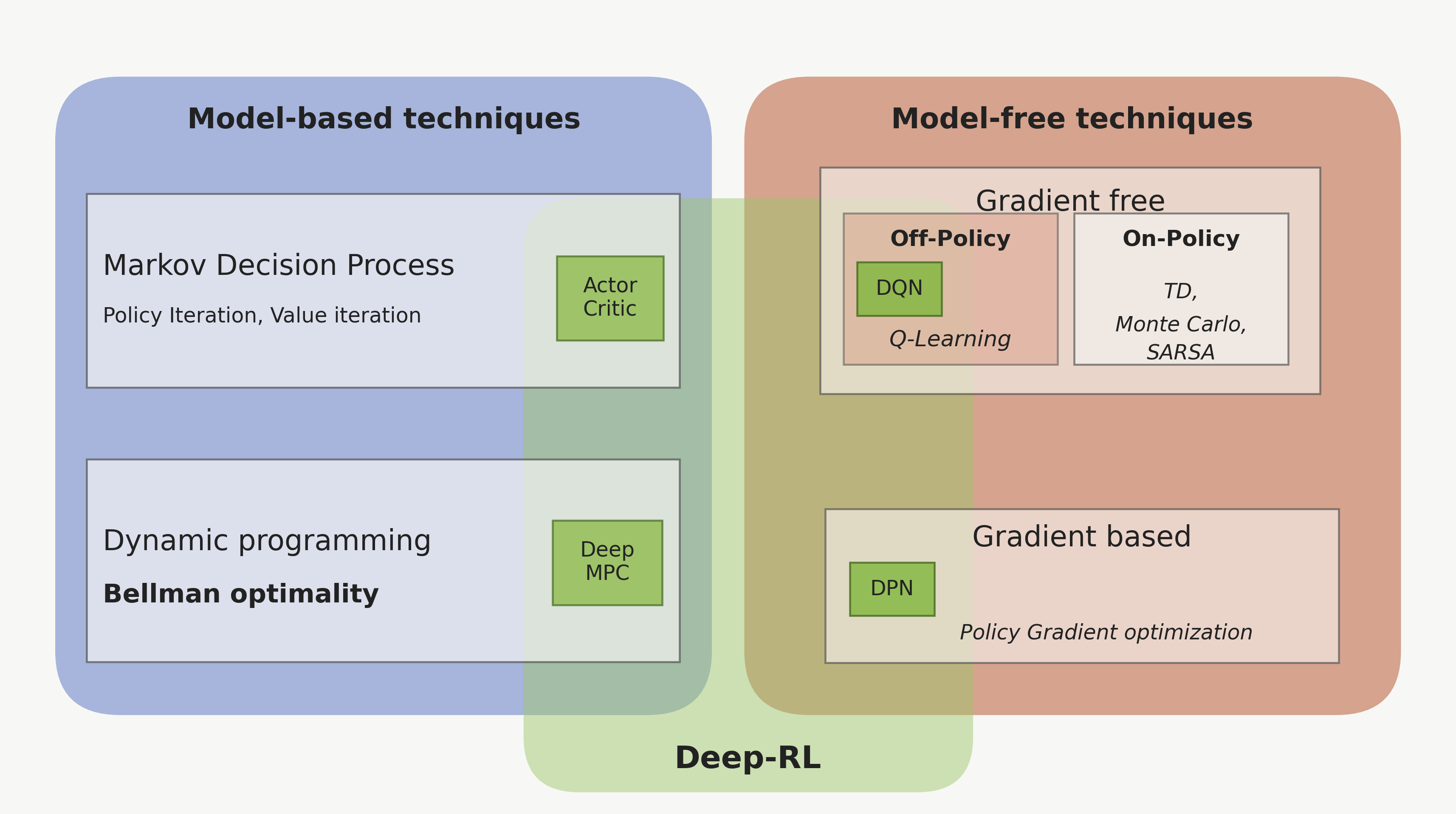
Model-free RL: Q-learning, SARSA, Policy Gradient
Finite State and Action Spaces: Restricted to discrete and countable sets, whereas real-world robotics and physical control tasks typically involve continuous states and actions.
Function approximation, Actor-Critic: DDPG, TD3, SAC, PPO
Curse of Dimensionality: Tabular value and policy storage scale exponentially as state dimensions grow (∣S∣×∣A∣), making high-dimensional environments (e.g., raw pixel inputs) computationally intractable.
Deep RL: neural approximation of V, Q, or π
Partial Observability: Assumes full access to the true ground-truth state (Ot=St), failing to account for real-world sensor noise, occlusions, and incomplete observations.
Actions that are taken has no influence on next observations. (Slot machines)
No delayed rewards.
RL problem with one state.
Examples:
Design of Clinical trials
Online ad suggestion, placement
Games
Web page personalization
Action now, Reward now.
Single State (St=S1).
Set of Actions = {A1,A2,...,An}.
Reward space = [0,1].
Learn a Stochastic Reward Function: Reward probabilities for actions are unknown in advance, so they must be learned stochastically through trial and error.
How to maximize PayOff among hundreds thousands of ads?
CTR, ClickThroughRate: Probability that users click on the ad.
Payment Rate: Money paid by the advertiser for each click.
Arms: {Ad1,Ad2,...,Adn}
Rewards: {0:No Click,1:Click}
Assuming a uniform payment of $1 for all ads, maximizing revenue simplifies to accurately estimating the Click-Through Rate (CTR).
Exploration vs. Exploitation: Should we display new ads with unknown CTRs to test them (Exploration), or continuously show top-performing ads with the highest historical CTR (Exploitation)?
No known optimal solution, but there are many heuristic approaches to balance exploration and exploitation.
used to balance between exploiting known good actions and exploring potentially better actions.
Optimism in the face of uncertaintiy: It will choose actions systematically that have a high potential for being optimal based on both their estimated value and their uncertatity.
The uncertainty bonus represents the value of exploring that arm.
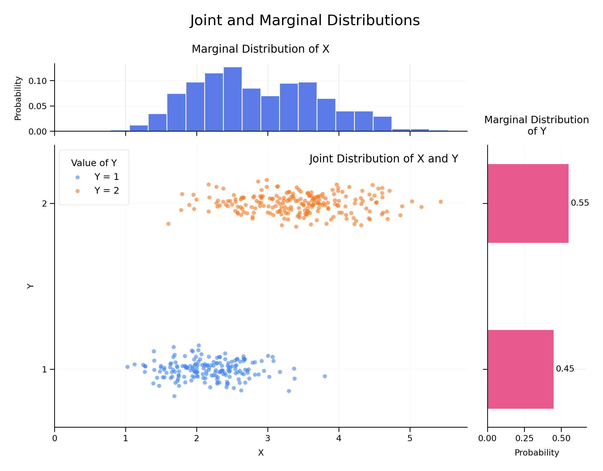
if X is continuous, then FX(x) is continuous and differentiable almost everywhere. The probability density function (pdf) is defined as:
fX(x)=dxdFX(x)
if X is discrete, then FX(x) is a step function and the probability mass function (pmf) is defined as:
pX(xi)=P(X=xi)
Central Limit Theorem: the distribution of the sum (or average) of a large number of independent, identically distributed variables will be approximately normal, regardless of the underlying distribution.
It outputs a real number that represents the length or size of a vector in a vector space.
x=(x1,x2,…,xn)↦f(x)=∥x∥
Non-negativity: ∀x∈Rn,∥x∥≥0
Definiteness: f(x)=0⟺x=0
Homogeneity: ∀x∈Rn,∀t∈R,f(tx)=∣t∣f(x)
Triangle inequality: ∀x,y∈Rn,f(x+y)≤f(x)+f(y)
∥x+y∥≤∥x∥+∥y∥
A norm is non-negative, only the zero vector has a norm of zero, scaling a vector by two doubles its norm, and the direct distance cannot be greater than the detoured distance.
∥x∥p=(∑i=1n∣xi∣p)p1,p≥1
L1 norm: ∥x∥1=∑i=1n∣xi∣
Manhattan distance.
L2 norm: ∥x∥2=∑i=1n∣xi∣2
Euclidean distance.
L-infinity norm: ∥x∥∞=maxi∣xi∣
∥(3,4)∥∞=max{3,4}=4
∥A∥F=∑i=1m∑j=1n∣aij∣2=tr(ATA)
Frobenius norm: A=[1324]
∥A∥F=12+22+32+42=30
It is the square root of the sum of the absolute squares of its elements.
A set of vertors X={x1,x2,...,xn} in a vector space V is said to spanV if every vector in V can be expressed as a linear combination of the vectors in X.
Span is the entire region that can be reached by scaling and adding the given vectors.
A set of vectors {v1,v2,...,vn} is said to be linearly independent if the only solution to the equation α1v1+α2v2+...+αnvn=0 is α1=α2=...=αn=0.
Column rank: The maximum number of linearly independent column vectors in a matrix.
Row rank: The maximum number of linearly independent row vectors in a matrix.
If one row vector is a combination of other row vectors, then it is linearly dependent.
The number of rows that are removed due to redundancy is the Rank of the matrix.
Due to the redundancy, the number of directions which is vanishing is the Nullity of the matrix.
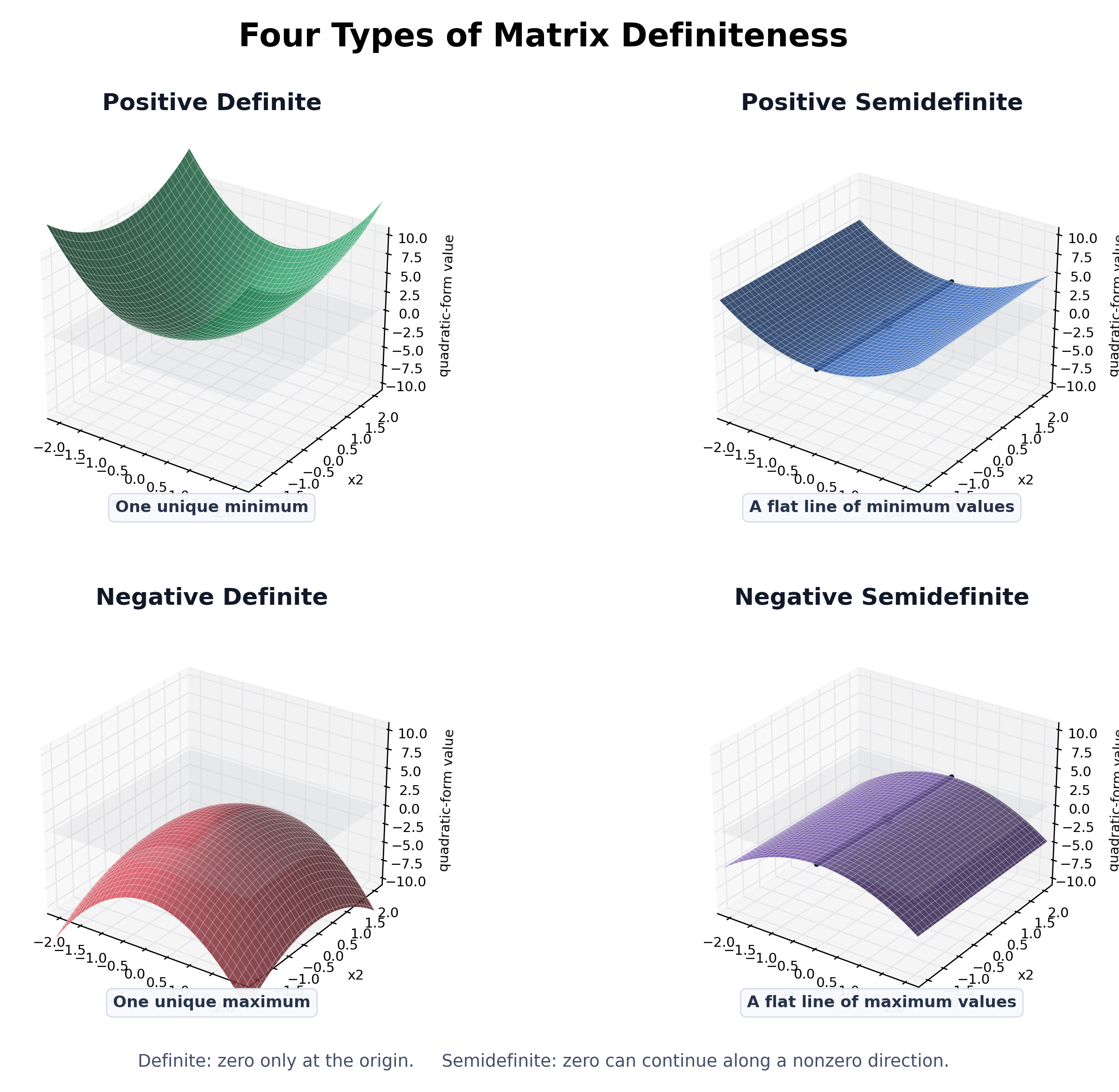
The quadratic form xTAx gives a scalar value that measures the cost, energy, or weighted magnitude of the vextor x, according to the quadratic surface defined by the matrix A.
Positive definite: Q(x)>0,∀x=0
Positive semi-definite: Q(x)≥0,∀x=0
Negative definite: Q(x)<0,∀x=0
Negative semi-definite: Q(x)≤0,∀x=0
Indefinite: Q(x) can be positive or negative for different x=0
행렬의 정부호성(양의 정부호, 양의 준정부호, 음의 정부호, 음의 준정부호, 부정정부호)
ATA=ATA⟹Q(x)=xTATAx=(Ax)T(Ax)=∥Ax∥2≥0
Always positive semi-definite because it is the square of the norm of the vector Ax.
A matrix A that appears complicated in the original coordinate system becomes the diagonal matrix Λ when expressed in the eigenvector coordinate system.
A=SΛS−1
In the eigenvector basis, the matrix A becomes the diagonal matrix Λ.
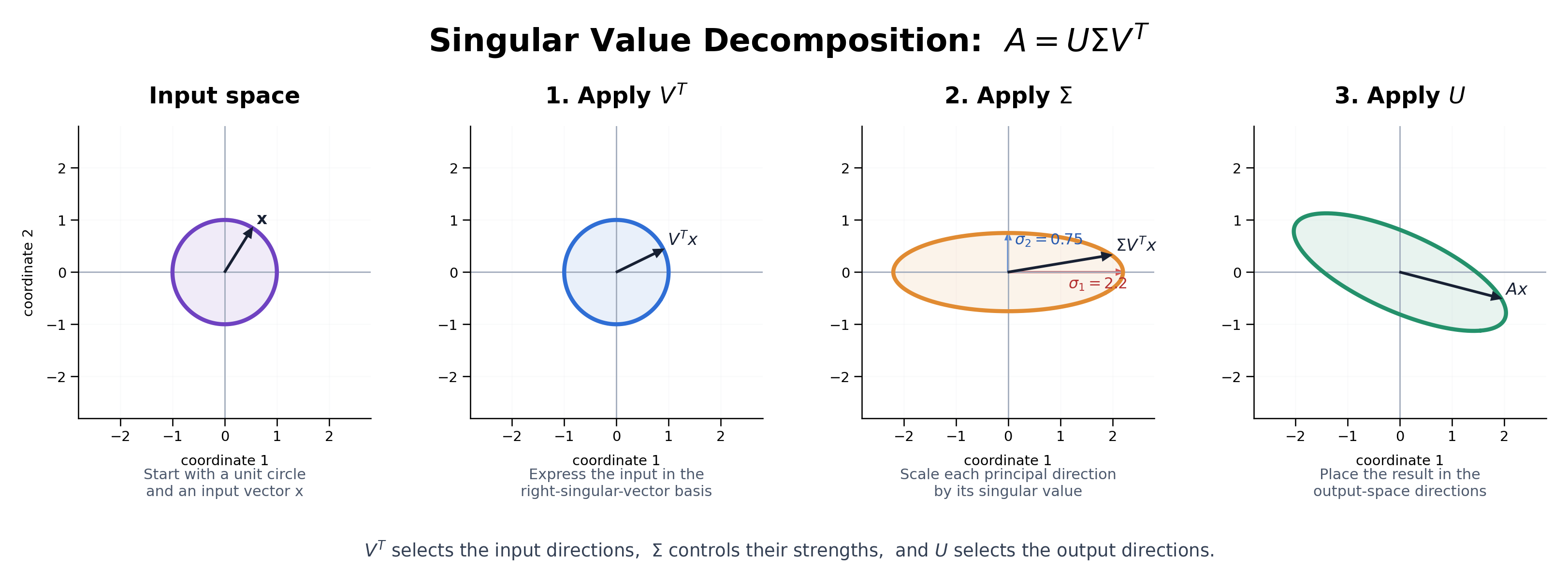
Diagonalization is generally defined for square matrices, while singular value decomposition can be applied to any rectangular or square matrix.
A=UΣVT
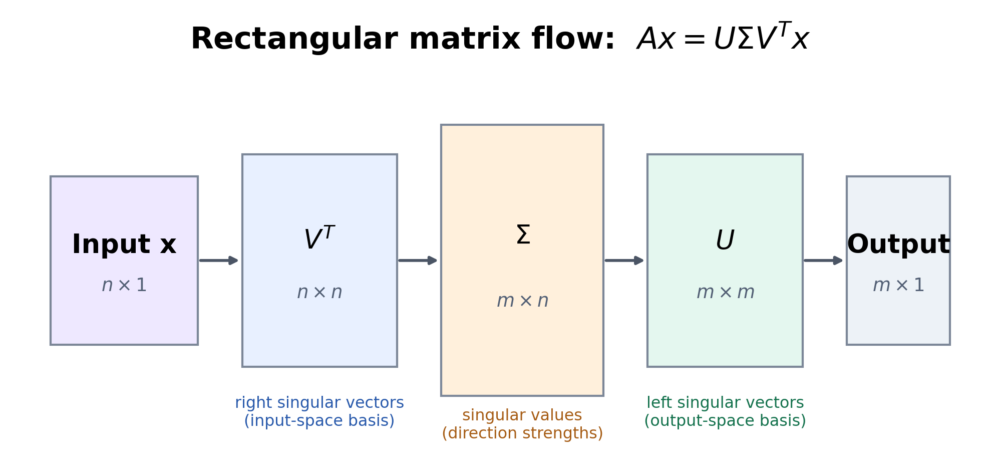
For A∈Rm×n,
U∈Rm×m,Σ∈Rm×n,V∈Rn×n
The columns of V are the right singular vectors and represent orthonormal directions in the input space.
The columns of U are the left singular vectors and represent orthonormal directions in the output space.
The diagonal entries of Σ are the singular values.
σ1≥σ2≥⋯≥0
For each singular-vector pair,
Avi=σiui
vi is an input direction.
σi is the scaling factor.
ui is the corresponding output direction.
The transformation A can be interpreted as three steps:
VT expresses the input in the right singular-vector basis.
Σ scales each direction by its singular value.
U maps the scaled result into the output space.
U and V are orthogonal matrices.
UTU=I,VTV=I
The singular vectors and singular values are related to the eigenvectors and eigenvalues of ATA and AAT.
ATAvi=σi2viAATui=σi2ui
The rank of A equals the number of nonzero singular values.
SVD is commonly used for dimensionality reduction, data compression, noise reduction, pseudoinverses, and latent-factor analysis.
n×1xVTn×1VTxΣm×1ΣVTxUm×1UΣVTx=m×1Ax
U is such that the m columns of U are the eigenvectors of AAT, known as the left singular vectors of A.
V is such that the n columns of V are the eigenvectors of ATA, known as the right singular vectors of A.
Σ is a rectangular diagonal matrix with each element being the square root of an eigenvalue of AAT or ATA.
SVD allows us to construct a lower rank approximation of a rectangular matrix.
Choose only the top r singular values in Σ.
The corresponding columns in U and rows in VT are also selected.
V represents the principal directions in the input space, U shows where those directions are mapped in the output space, and Σ shows how much each direction is scaled.