4 posts tagged with "IQC"

Boolean Functions​

$f: \{0,1\}^n \to \{0,1\}$

• $n=1$
• Constant: smae output for all inputs ($f_0$ and $f_3$).
• Balanced: outputs 0 for exactly half, 1 for the other half ($f_1$ and $f_2$).
• In the worst case, need $2^{n-1}+1$ quries to decide which type $f$ is exponetial in $n$.

The Quantum Oracle​

• Traditional Oracle: black box that computes $f$.
• Query complexity: number of queries to the oracle needed to solve a problem.

$x \xrightarrow{O_f} f(x)$

• Quantum Oracle: unitary operation that encodes $f$.

$U_f \ket{x}\ket{y} = \ket{x}\ket{y \oplus f(x)}$

• First register: input $x$.
• Second register: auxiliary qubit initialized to $\ket{0}$ or $\ket{1}$.
• Oracle don't change $x$, but flips $y$ if $f(x)=1$.
  • $0 \oplus 0 = 0$
  • $0 \oplus 1 = 1$
  • $1 \oplus 0 = 1$
  • $1 \oplus 1 = 0$
• $f(x) = 0$: $y$ unchanged.
• $f(x) = 1$: $y$ flipped.
• Example:
  • $\ket{x}\ket{0}$
  • $U_f \ket{x}\ket{0} = \ket{x}\ket{0} \oplus \ket{f(x)} = \ket{x}\ket{f(x)}$.
  • if $f(x) = 0$: $\ket{x}\ket{0}$.
  • if $f(x) = 1$: $\ket{x}\ket{1}$
• so that it ignores the input $x$ and only flips the second qubit if $f(x)=1$.
• it can be reversed: $(y \oplus f(x)) \oplus f(x) = y$.

Phase Kickback​

• Prepare the scratch qubit in $\ket{-} = \frac{1}{\sqrt{2}}(\ket{0} - \ket{1})$.
  • $U_f \ket{x}\ket{-} = \frac{1}{\sqrt{2}}(U_f \ket{x} \ket{0} - U_f \ket{x} \ket{1})$
  • $= \frac{1}{\sqrt{2}}(\ket{x} \ket{0 \oplus f(x)} - \ket{x}\ket{1 \oplus f(x)})$
  • if $f(x) = 0 \rightarrow \\ \frac{1}{\sqrt{2}}(\ket{x}\ket{0 \oplus 0} - \ket{x}\ket{1 \oplus 0}) \\ = \frac{1}{\sqrt{2}}(\ket{x}\ket{0} - \ket{x}\ket{1}) \\ = \ket{x} \frac{1}{\sqrt{2}}(\ket{0} - \ket{1}) \\ = \ket{x}\ket{-}$.
  • if $f(x) = 1 \rightarrow \\ \frac{1}{\sqrt{2}}(\ket{x}\ket{0 \oplus 1} - \ket{x}\ket{1 \oplus 1}) \\ = \frac{1}{\sqrt{2}}(\ket{x}\ket{1} - \ket{x}\ket{0}) \\ = - \ket{x} \frac{1}{\sqrt{2}}(\ket{0} - \ket{1}) \\ = -\ket{x}\ket{-}$.
    • it doesn't matter where the phase is, it can be moved around:
    • $\alpha(\ket{\psi} \otimes \ket{\phi}) = \alpha\ket{\psi} \otimes \ket{\phi} = \ket{\psi} \otimes \alpha\ket{\phi}$.
• if we put the second register to $\ket{-}$, $f(x)$ will be encoded in the phase of the first register.

$\ket{x}\ket{-}\mapsto (-1)^{f(x)} \ket{x} \ket{-}$

• The function's output has been "kicked back" into the phase of the first register, while the second register remains unchanged.

The Deutsch Problem​

• Given a boolean function $f:\{0,1\}^{n} \to \{0,1\}$, determine if $f$ is constant or balanced.
• Constant: same output for all inputs.
• Balanced: outpus 0 for half the inputs and 1 for the other half.

1. Prepare $\ket{0}\ket{1}$.
2. Apply $H$ to both qubits $\to \ket{+}\ket{-}$.
3. Apply oracle $U_f$.
4. Phase kickback encodes $f$ in the input phase.
5. Apply $H$ to input qubit, then measure.

• One query to the oracle is sufficient to determine if $f$ is constant or balanced.
• if measure 0: $f$ is constant.
• if measure 1: $f$ is balanced.

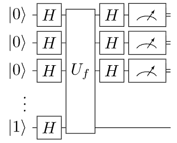
Deustch-Jozsa Algorithm​

The direct generalization for any $n$-bit boolean function.

1. Input register $n$ qubits: Initialize qubits in $\ket{0}$ and apply $H$ gate to each one.
2. Scratch Qubit $1$ qubit: Initialize in $\ket{1}$ with $X$ and then apply an $H$ gate.
3. Oracle: Apply $U_f$ to the input and scratch registers (All qubits).
4. Final Hadamards: Apply $H$ to input qubits.
5. Measurement: Measure the input register.

• if all qubits returned $0$: $f$ is constant.
• if any qubit returned $1$: $f$ is balanced.

How it works​

• The initial state is

$\ket{00 \cdots 0} \ket{1}$

• After applying $H$ gates to the input and scratch registers, we get

$\ket{00 \cdots 0} \rightarrow \frac{1}{\sqrt{2^n}} \left( \ket{00 \cdots 0} + \ket{00 \cdots 1} + \cdots + \ket{11 \cdots 1} \right)$

• The input register is in a superposition of a computational states containing all possible inputs to $n$-bit string.
• The last qubit hasn't changed from $n = 1$ case, so it is in the state $\ket{-}$.
  • $H\ket{1} = \ket{-}$
• The definition of the oracle was generic for any bit string: $U_f \ket{x}\ket{-} = (-1)^{f(x)} \ket{x} \ket{-}$
• The phase-kickback puts a phase in front of each term in the input register that depends on the output of the function $f$: $\frac{1}{\sqrt{2^n}}\big(\;(-1)^{f(00\ldots0)}|00\ldots 0\rangle+ \cdots +(-1)^{f(11\ldots1)}|11\ldots 1\rangle\;\big)$
  • The scratch qubit remains in $\ket{-}$, so we can ignore it for the rest of the algorithm.
• Constant case
  • if $f$ is constant, then all the phases are the same, either $+1$ or $-1$:
  • $f(00 \cdots 0) = f(00 \cdots 1) = \cdots = f(11 \cdots 1) = 0$
  • $f(00 \cdots 0) = f(00 \cdots 1) = \cdots = f(11 \cdots 1) = 1$
  • The phse in front of every computational state is the same, Either $+1$ or $-1$.
  • Before the second application of the $H$ gates, the state of the input register is:
  • $\pm \frac{1}{\sqrt{2^n}} \left( \ket{00 \cdots 0} + \ket{00 \cdots 1} + \cdots + \ket{11 \cdots 1} \right)$
  • In measurement, in either case, the probability to obtain $P(00 \cdots 0) = 1$
  • A constant function deterministically returns all zeros with a single query.
• Balanced case
  • we are promised the function is either constant or balanced, so there are equal number of $+1$ and $-1$ phases. so we don't need to consider this case.
  • If the measurement produces anything but all zeros, we know with certainty the function is not constant, so it must be balanced.
  • There are a lot of balanced function, but half the terms in the superposition will exactly have a $-1$ phase.
  • It's clearly orthogonal to the state with all ones in superposition.
  • Appllying $H$'s will change the state to some other superpostiion, or perhaps a unique computational state.
  • But, orthogonality to $\ket{00 \cdots 0}$ must remain.
  • A balenced function deterministically returns a state with at least one entry as $1$, with a single query.

One quantum query vs $2^{n-1} + 1$ classical queries. It is an algorithm that puts all inputs into superposition at once, encodes the function values as phases, and then uses interference to distinguish between constant and balanced functions.

Buildling Oracles​

Multi-Controlled and Anti-Controlled Gates​

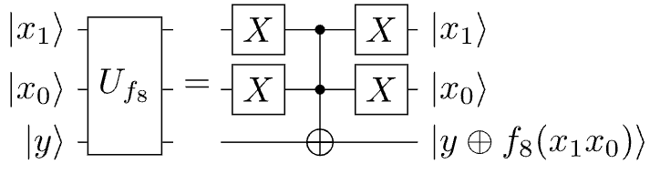
• build $U_f$ that applies $X$ to the output qubit exactly when $f(x) = 1$.
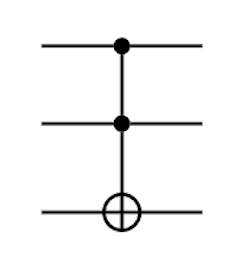
  • if $n=2$, the multi-controlled $X$ gate is a Toffoli gate.
  • $x=11$ is the only input that gives $f(x) = 1$, so we can use a Toffoli gate with controls on the first two qubits and target on the output qubit.
    • This is because the Toffoli gate will flip the output qubit if and only if both control qubits are $\ket{1}$, which corresponds to the input $x=11$.
  • if $x=00$ is the only input that gives $f(x) = 1$, we can use an anti-controlled Toffoli gate, which applies $X$ to the target qubit if both control qubits are $\ket{0}$.
    • This is because the anti-controlled Toffoli gate will flip the output qubit if and only if both control qubits are $\ket{0}$, which corresponds to the input $x=00$.
    • Applying $X$ gates to the two control qubits, then applying a Toffoli gate, and then applying $X$ gates again to the control qubits will effectively create an anti-controlled Toffoli gate.

• A multi-controlled $X$ gates ($C^nX$) flips the target only all control qubits are $\ket{1}$.
• To target a specific input $x$:
  • Place $X$ gates on each qubit $i$ where $x_i = 0$. (anti-control)
  • Apply $C^nX$.
  • Undo the $X$ gates.
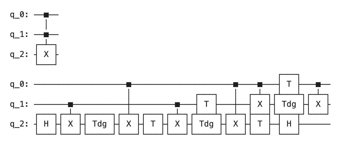
• For $n$ qubits, it can be generalized to perform an $X$ gate (or any $U$) with $n$ control qubits, requireing $n-1$ extra scratch qubits and $2(n-1)$ Toffoli gates.
• Whenever scratch qubits are invoked, always see a symmetric pattern of gates.
• $U_{f8} U_{f1} \ket{x}\ket{y} = \ket{x}\ket{y \oplus f_1(x) \oplus f_8(x)} = \ket{x}\ket{y \oplus f_9(x)}$

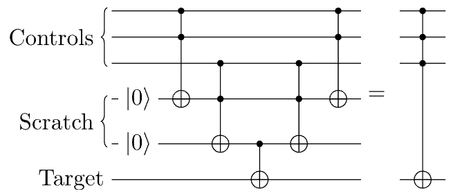
1. The computation is done using the scratch qubits.
2. The answer is copied to the target or output register
3. The computation is inverted to reset the scratch qubits to $\ket{0}$.

• called "uncomputation", ensures the scratch qubits are returned to their initial state.
• no input or output qubits are entangled with the scratch qubits at the end of the algorithm.

Implementing Deutsch-Jozsa​

def random_oracle(n):
    # Circuit object to hold the gates
    circuit = qiskit.QuantumCircuit(n + 1)

    # With 50% probability, return a constant oracle
    if np.random.randint(0, 2):
        qasm = ""
        # another 50:50 chance of it being a 1 instead of 0 oracle
        if np.random.randint(0, 2):
            qasm += f"x q[{n-1}];"
        return qasm, "constant"

    # A balanced function has half the inputs as 0
    # Randomly select where those are
    zero_strings = np.random.choice(range(2**n),int(2**(n-1)),replace=False)

    for string in zero_strings:

        # Convert base 10 to 2
        bitstring= f"{string:0b}"

        # X gates for 0 locations
        for xi, bit in enumerate(reversed(bitstring)): # enumerate iterates through the list as well as the index in the list
            if bit == "1":
                circuit.x(xi)

        # C^n X gate
        circuit.mcx(list(range(n)), n)

        # X gates for 0 locations
        for xi, bit in enumerate(reversed(bitstring)):
            if bit == "1":
                circuit.x(xi)

    transpiled_circuit = qiskit.transpile(circuit, basis_gates=["u1", "u3", "u2", "cx"])
    qasm = qiskit.qasm2.dumps(transpiled_circuit)[47:]
    return qasm, "balanced"

OPENQASM 2.0;
qreg q[3];
creg c[2];

x q[2];
h q[0];
h q[1];
h q[2];

/* oracle for f(00)=1 */
x q[0];
x q[1];
ccx q[0],q[1],q[2];
x q[0];
x q[1];

/* oracle for f(11)=1 */
ccx q[0],q[1],q[2];

h q[0];
h q[1];

measure q[0] -> c[0];
measure q[1] -> c[1];

OPENQASM 2.0;
qreg q[n+1];
creg c[n];

x q[n];
h q[0];
h q[1];
...
h q[n];
/* oracle U_f */
h q[0];
h q[1];
...
h q[n-1];
measure q[0] -> c[0];
...
measure q[n-1] -> c[n-1];

Bernstein-Vazirani Algorithm​

• Given $f_s: \{0,1\}^n \to \{0,1\}$ defined as $f_s(x) = s \cdot x \mod 2$
  • where $s$ is an unknown $n$-bit string and $x$ is the input.
• The goal is to determine the hidden string $s$ as few queries as possible.
• Classically: query $f$ with input $e_0 = 00 \cdots 01$, $e_1 = 00 \cdots 10$, ..., $e_{n-1} = 10 \cdots 00$ to get each bit of $s$.
  • Total $n$ queries.
• Quantum: use the exact same circuit as Deutsch-Jozsa.
  • $U_{f_s} \ket{x} = (-1)^{s \cdot x} \ket{x}$.
    • where we can ignore the output register in the $\ket{-}$ state.
    • For $n =1$, the state after the oracle before the final $H$ gate is:
      • $\frac{1}{\sqrt{2}} \left( \ket{0} + (-1)^{s} \ket{1} \right)$
    • which is $\ket{+}$ if $s=0$ and $\ket{-}$ if $s=1$.
  • Applying $H$ to this state returns $s$:
    • $H \frac{1}{\sqrt{2}} \left( \ket{0} + (-1)^{s} \ket{1} \right) = \ket{s}$.
  • The measurement deterministically reveals $s$.

n=2 case​

• $s = s_1s_0$ and $x = x_1 x_0$
• $\rightarrow s\cdot x = s_1x_1 + s_0 x_0$

this factorized into:

$\frac{1}{\sqrt{2}}\big(\ket 0 + (-1)^{s_1}\ket 1\big)\otimes \frac{1}{\sqrt{2}}\big(\ket 0 + (-1)^{s_0}\ket 1\big).$

this reduces the same agument as $n=1$ for each qubit where after the final $H$ gates, the state becomes:

Implemnting Bernstein-Vazirani​

• $\mathbb{I}$ if $s = 0$ and $CNOT$ if $s = 1$.
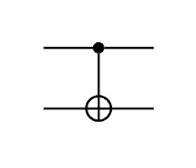
• To implement $f_{s}(x) = s \cdot x$, we can use a CNOT from qubit $i$ to the scratch qubit if $s_i = 1$.

import numpy as np
from qiskit import QuantumCircuit, transpile
from qiskit_aer import AerSimulator


def bv_query(n, secret=None):
    # Build oracle for f_s(x) = s · x
    # q[0]..q[n-1] = input register
    # q[n] = scratch/output qubit

    if secret is None:
        value = np.random.randint(0, 2 ** n)
        secret = format(value, f"0{n}b")
    else:
        secret = secret.zfill(n)

    oracle = QuantumCircuit(n + 1, name="Uf")
    for index, bit in enumerate(reversed(secret)):
        if bit == "1":
            oracle.cx(index, n)

    return oracle, secret


def bernstein_vazirani_circuit(n, secret=None):
    # Build full Bernstein-Vazirani circuit
    oracle, secret = bv_query(n, secret)

    qc = QuantumCircuit(n + 1, n)

    # Prepare scratch qubit in |->
    qc.x(n)

    # Apply Hadamards to all qubits
    for i in range(n + 1):
        qc.h(i)

    # Apply oracle
    qc.compose(oracle, inplace=True)

    # Apply final Hadamards to input register
    for i in range(n):
        qc.h(i)

    # Measure input register
    for i in range(n):
        qc.measure(i, i)

    return qc, secret


def run_bernstein_vazirani(n, secret=None, shots=1):
    qc, secret = bernstein_vazirani_circuit(n, secret)

    simulator = AerSimulator()
    compiled = transpile(qc, simulator)
    result = simulator.run(compiled, shots=shots).result()
    counts = result.get_counts()

    measured = max(counts, key=counts.get)
    recovered = measured[::-1]

    return qc, secret, recovered, counts


# Example
qc, secret, recovered, counts = run_bernstein_vazirani(5, "01101")
print(qc.draw())
print("Secret   :", secret)
print("Measured :", recovered)
print("Counts   :", counts)

OPENQASM 2.0;
qreg q[6];
creg c[5];

x q[5];
h q[0];
h q[1];
h q[2];
h q[3];
h q[4];
h q[5];

cx q[0],q[5];
cx q[2],q[5];
cx q[3],q[5];

h q[0];
h q[1];
h q[2];
h q[3];
h q[4];

measure q[0] -> c[0];
measure q[1] -> c[1];
measure q[2] -> c[2];
measure q[3] -> c[3];
measure q[4] -> c[4];

Summary​

• There are $2^{2^n}$ possible Boolean functions from $\{0,1\}^n$ to $\{0,1\}$.
• A Boolean function is balanced if it outputs 1 on exactly half of the inputs, that is, on $2^{n-1}$ out of the $2^n$ possible inputs.
• In Deutsch’s algorithm with $n=1$, only 1 quantum query is needed to distinguish a constant function from a balanced function.
• A quantum oracle for $f$ is defined as the unitary $U_f:\ |x\rangle|y\rangle \mapsto |x\rangle|y\oplus f(x)\rangle.$
• Every XOR-based function of the form $f(x)=x_j\oplus x_k\oplus\cdots$ that depends on at least one input bit is balanced.
• Using multi-controlled $X$ gates, together with anti-controls when needed, we can implement an oracle for any Boolean function.
• The phase kickback multiplies the state by the phase factor $(-1)^{f(x)}$, so the phase changes exactly when $f(x)=1$.
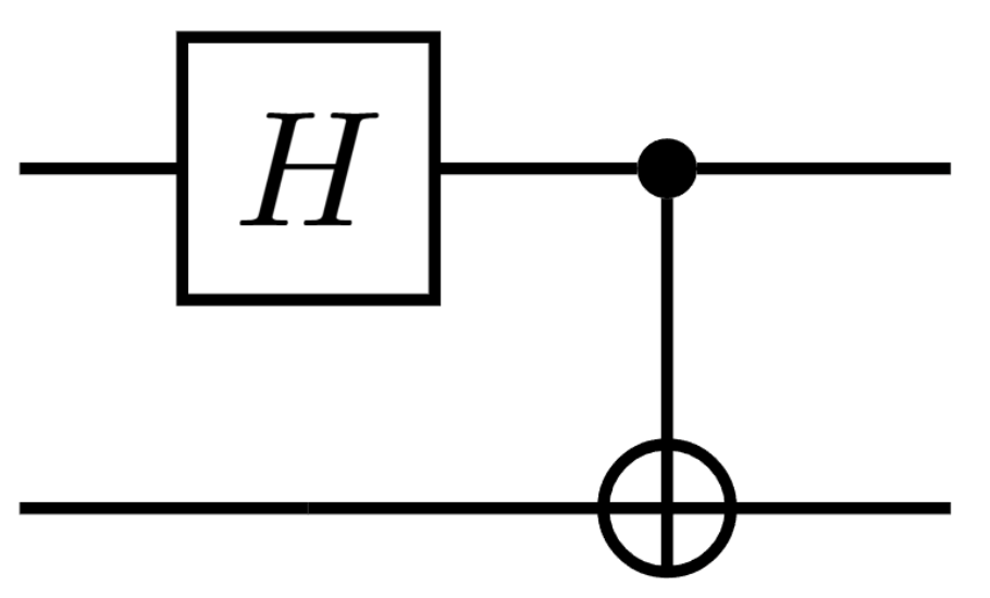
• If these questions were stored in a Python list called questions, then the 8th question would be questions[7].
• Applying Hadamard gates to $n$ qubits initialized in $|0\rangle$ produces an equal superposition over all $2^n$ computational basis states.
• In Deutsch–Jozsa for $n>1$, measuring all input qubits as 0 means that $f$ is constant.
• Bernstein–Vazirani solves the hidden-string problem $f(x)=s\cdot x$ with 1 quantum query.
• A multi-controlled $X$ gate with 3 controls can be implemented using scratch qubits and 4 Toffoli gates.
• Applying $U_{f_1}$ followed by $U_{f_2}$ yields an oracle whose action on the scratch qubit corresponds to $f_1(x)\oplus f_2(x)$.
• Uncomputation resets scratch qubits to their initial states by applying the inverse of the computation, which means reversing the order of the steps.
• Multi-controlled gates with more than one control can be decomposed into simpler gates, but in general this requires more than just $CX$ and $X$; single-qubit gates are also needed.

Superdense Coding​

• counterintuitive protocol that allows us to send 2 bits of classical information by sending only 1 qubit, using pre-shared entanglement
• it's often contextualized as a game with Alice and Bob.
• Alice and Bob share and entangled pair of qubits
• Pre-shared Entanglement (Shared Bell pair)
  • $|\Phi^+\rangle = \frac{1}{\sqrt{2}}(|00\rangle + |11\rangle)$
• Alice wants to send 2 bits of classical information (00, 01, 10, or 11) to Bob
  • For 00: Apply Identity $I$ (do nothing)
  • For 01: Apply Pauli-X $X$ (bit flip)
  • For 10: Apply Pauli-Z $Z$ (phase flip)
  • For 11: Apply $XZ$ (bit and phase flip)
• Alice sends her one qubit to Bob (Bob possesses both qubits of the entangled pair)
• Bob decodes the information
  • Inverts the entanglement operation on the two qubits (CNOT followed by Hadamard)
  • Measures each of the qubits
  • The outcome of this measurement reveals the two bits Alice encoded.
• $|\Phi^+\rangle$: is the most common and convenient form (Bell State) of entanglement and is also maximally entangled state despite single-qubit unitary gates.
  • Easy to build circuits for it
  • Symmetric and has nice properties that make it ideal for protocols like superdense coding and teleportation
  • Other Bell states can be generated from $|\Phi^+\rangle$ by applying single-qubit gates.

Superdense Coding Circuit​

• Alice's message $mn$, where each of $m$ and $n$ is a bit (0 or 1)
• Alice's operation can be represented as $Z^m X^n \otimes \mathbb{I} | \Phi^+\rangle$
  • $m=0 \Rightarrow Z^0 = I$ (no phase flip)
  • $m=1 \Rightarrow Z^1 = Z$ (phase flip)
  • $n=0 \Rightarrow X^0 = I$ (no bit flip
  • $n=1 \Rightarrow X^1 = X$ (bit flip)
  • $00 \rightarrow I$
  • $01 \rightarrow X$
  • $10 \rightarrow Z$
  • $11 \rightarrow ZX$
• $Z^m|b\rangle = (-1)^{mb}|b\rangle$ (phase flip)
• $X^n|a\rangle = |a \oplus n\rangle$ (xor operation)

$X^n \left(\frac{1}{\sqrt{2}} (|00\rangle + |11\rangle)\right) = \frac{1}{\sqrt{2}} \left( |n0\rangle + |(1\oplus n)1\rangle \right)$

• $n=0$: $\frac{1}{\sqrt{2}} (|00\rangle + |11\rangle) = |\Phi^+\rangle$
• $n=1$: $\frac{1}{\sqrt{2}} (|10\rangle + |01\rangle)$

$Z^m X^n \left(\frac{1}{\sqrt{2}} (|00\rangle + |11\rangle)\right) = \frac{1}{\sqrt{2}} \left( (-1)^{mn}|n0\rangle + (-1)^{m(1\oplus n)}|(1\oplus n)1\rangle \right)$

• $|n0\rangle$: first qubit is $n$, $(-1)^{mn}$ is the phase factor
• $|(1\oplus n)1\rangle$: first qubit is $1\oplus n$, $(-1)^{m(1\oplus n)}$ is the phase factor
• Bob's decoding operation is the inverse of the entanglement operation
  • $CNOT |a\rangle |b\rangle = |a\rangle |a \oplus b\rangle$

• which is seperable state.
• First qubit is $|n\rangle + (-1)^m|1 \oplus n\rangle$ and second qubit is $|n\rangle$.
• $n, m \in \{0, 1\}$, then apply Hadamard to the first qubit:

• second qubit is $|n\rangle$, so the final state is:

$(-1)^{mn}(-1)^{nm}|m\rangle|n\rangle = |mn\rangle$

Superdense QASM​

OPENQASM 2.0;
qreg q[2];
creg c[2];

// Prepare Bell pair
h q[0];
cx q[0],q[1];

// Alice's encoding
// For message 11: apply X and Z
x q[0];
z q[0];

// Alice sends q[0] to Bob (in simulation, we just proceed)

// Bob's decoding
cx q[0],q[1];
h q[0];

// Measure both qubits
measure q[0] -> c[0];
measure q[1] -> c[1];

QASM Programming​

Custom Gates​

// params: parameters for the gate (e.g., rotation angles)
// q_args: quantum arguments (qubits the gate acts on)
gate NAME(parameters) q_args {
  // Define gate operations
}

gate bell a,b {
  h a;
  cx a,b;
}

qreg q[2];
creg c[2];

// Use the custom bell gate
bell q[0], q[1];

// Measure the qubits
measure q[0] -> c[0];
measure q[1] -> c[1];

Toffoli Gate​

// Toffoli gate (CCX)
gate ccx a, b, c {
  h c;
  cx b, c;
  tdg c;
  cx a, c;
  t c;
  cx b, c;
  tdg c;
  cx a, c;
  t b;
  t c;
  cx a, b;
  h c;
  t a;
  tdg b;
  cx a, b;
}

Rotation Gates​

// Rotation around Y-axis
gate ry_deg(theta) q {
  ry(theta/180 * pi) q;
}

// Rotation around X-axis
gate rx_deg(theta) q {
  rx(theta/180 * pi) q;
}

Qiskit​

IBM

import qiskit

superdense = qiskit.QuantumCircuit(2, 2)
superdense.draw()

superdense.h(0)
superdense.cx(0, 1)
superdense.draw()

# Alice's encoding for message '11'
superdense.x(0)
superdense.z(0)
superdense.draw()

# Bob unentangles the two qubits (reverses the entangling gate)
superdense.cx(0,1)
superdense.h(0)

# The measurement pattern is `measure(qubit to measure, classical bit to store result)`
superdense.measure(0,0)
superdense.measure(1,1)
superdense.draw()

from qiskit.providers.basic_provider import BasicSimulator

sim = BasicSimulator()
# run the circuit on the simulator with 1 shot (execute the circuit once)
result = sim.run(superdense, shots=1).result().get_counts()

print(result)
# {'11': 1}

Custom Gates in Qiskit​

bell = qiskit.QuantumCircuit(2, name='bell')
bell.h(0)
bell.cx(0, 1)
bell_gate = bell.to_gate()

c = qiskit.QuantumCircuit(2)
c.append(bell_gate, [0, 1])
c.draw()

Decompose a custom gate​

ccxgate = qiskit.circuit.library.CCXGate()
ccx = qiskit.QuantumCircuit(3)
ccx.append(ccxgate, [0, 1, 2])

print(ccx)
print(ccx.decompose())

Cirq​

Google

import cirq

alice = cirq.NamedQubit('Alice')
bob = cirq.NamedQubit('Bob')

superdense = cirq.Circuit()
superdense.append([
  cirq.H(alice),
  cirq.CNOT(alice, bob),
])

superdense.append([
  cirq.X(alice),
  cirq.Z(alice),
])

superdense.append([
  cirq.CNOT(alice, bob),
  cirq.H(alice),
])

superdense.append(cirq.measure(alice, bob, key='received'))

print(superdense)

simulator = cirq.Simulator()
result = simulator.run(superdense, repetitions=1)
print(result)
# received=1, 1

Pennylane​

Xanadu

import pennylane as qml

def entangle():
    qml.Hadamard(wires=0)
    qml.CNOT(wires=[0, 1])

print(qml.draw(entangle)())

device = qml.device("default.qubit", wires=[0, 1])

# Wrap the quantum function as a QNode
entangle_qnode = qml.QNode(my_circuit, device)

# Set the number of shots to 10
entangle_qnode = qml.set_shots(entangle_qnode, shots=10)

import numpy as np

state = np.array([1, 1j], dtype=complex)

state = state / np.linalg.norm(state)

def teleport(state):
    # Ensure "state" is loaded into the first qubit
    # (otherwise qubits would start in |0>)
    qml.StatePrep(state, wires=0)

    # Shared entanglement between qubits 1 and 2
    qml.Hadamard(wires=1)
    qml.CNOT(wires=[1, 2])

    # Alice's operation:
    # CNOT from Alice's input qubit to her half of the Bell pair,
    # then Hadamard on the input qubit
    qml.CNOT(wires=[0, 1])
    qml.Hadamard(wires=0)

    # Measurement (store the classical outcomes)
    m0 = qml.measure(0)
    m1 = qml.measure(1)

    # Bob's conditional correction operations
    qml.cond(m1, qml.PauliX)(wires=2)
    qml.cond(m0, qml.PauliZ)(wires=2)

    # Return Bob's qubit as a density matrix
    return qml.density_matrix(wires=2)

print(qml.draw(teleport)(state))

Quantum Teleportation​

• if there is entanglement:
  • we can use it to send 2 bits of classical information by sending 1 qubit (superdense coding)
  • we can use it to send 1 qubit of quantum information by sending 2 bits of classical information (teleportation)
• Alice wants to send a qubit $|\psi\rangle = \alpha|0\rangle + \beta|1\rangle$ to Bob, but only has a classical channel.

Protocol​

1. Alice and Bob share $|\Phi^+\rangle$ (pre-shared entanglement)
2. Alice applies $CNOT$ (her qubit -> her Bell half), then $H$, then measures both, obtaining 2 classical bits (00, 01, 10, or 11)
3. Alice sends $mn$ classically to Bob
4. Bob applies $X^n Z^m$ to his qubit, recovering $|\psi\rangle$

• For 00: Apply Identity $I$ (do nothing)
• For 01: Apply Pauli-X $X$ (bit flip)
• For 10: Apply Pauli-Z $Z$ (phase flip)
• For 11: Apply $XZ$ (bit and phase flip)
• Bob now has a qubit in the state Alice wanted to send $|\psi\rangle$ without Alice ever sending a qubit directly to Bob.

Teleportation Circuit​

$|\psi\rangle \otimes |\Phi^+\rangle = \left(\alpha |0\rangle + \beta |1\rangle\right) \otimes \frac{1}{\sqrt{2}} \left(|00\rangle + |11\rangle\right)$

$|\psi\rangle \otimes |\Phi^+\rangle = \frac{1}{\sqrt{2}} \left(\alpha |0\rangle |00\rangle + \alpha |0\rangle |11\rangle + \beta |1\rangle |00\rangle + \beta |1\rangle |11\rangle\right)$

• Alice applies a $CNOT$ gate with her qubit $|\psi\rangle$ as control and her half of the Bell pair $|\Phi^+\rangle$ as target.
  • $\beta |1\rangle |00\rangle$ becomes $\beta |1\rangle |10\rangle$ (target flips when control is 1)
  • $\beta |1\rangle |11\rangle$ becomes $\beta |1\rangle |01\rangle$ (target flips when control is 1)

$\frac{1}{\sqrt{2}} \Big(\alpha |0\rangle |00\rangle + \alpha |0\rangle |11\rangle + \beta |1\rangle |10\rangle + \beta |1\rangle |01\rangle\Big)$