11 posts tagged with "fda"

Bias​

• Bias quantifies how much on average the predicted values differ from the actual values.
• High bias implies the model is under-performing.

Variance​

• Variance quantifies how sensitive the model is to small changes in the training samples.

Ensemble Methods​

• The intuition behind ensemble methods is to decrease bias and variance by using multiple machine learning algorithms.
• Any machine learning algorithm can be used in ensemble methods.
  • decision trees, neural networks, logistic regressions, etc.
• Base models are as diverse as possible.
• Train each base model to predict as accurately as possible.

Sequential ensemble methods​

• Arrange weak learners in a sequence, such that weak learners learn from next learner in the sequence to create better predictive models.
• Each model fits the residual of its predecessor.

Parallel ensemble methods​

• to use different variations of the same dataset, of the smae classifier, and aggregate the results.

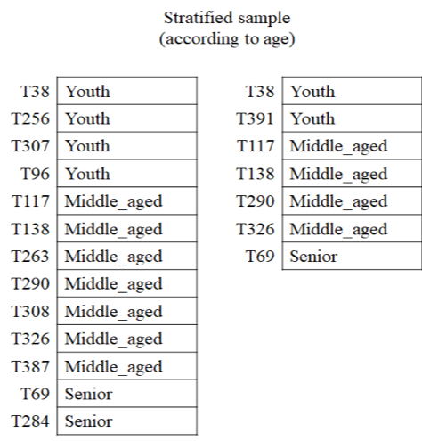
Bootstraping​

• Sampling technique that creates multiple subsets of datasets from the original dataset.
• when inferring results for a population from results found on a collection of smaller random samples of that population.

Bagging​

Bootstrap aggregating

• Generates subsets (bags) of traning data by sampling from the original training dataset with replacement.
• To overcome the complexity of models that overfit the training data.

Boosting​

• fits multiple models sequentially
• each model in the sequence is fitted giving more weight to the data points that were poorly handled by the previous models in the sequence.
• This process is iterated until the error function does not change, or the maximum limit of the number of estimators is reached.

Random Forest​

• Shallow trees have lower variance and higher bias, whereas deep trees have low bias but high variance.
  • Shallow trees are chosen for sequential ensemble methods
  • Deep trees are chosen for bagging methods (or parallel ensemble methods).
• a bagging method where deep trees are used and fitted on bootstrap samples, and then combined to produce an output with lower variance.
• selects randomly a set of features which are then used to decide the best split at each node of the tree.
• can be applied to both regression and classification tasks.
• can learn binary features, categorical features and numerical features.

1. create from the original dataset multiple bootstrap samples.
2. at each node in the decision tree, a random set of features is considered to decide the most beneficial split.
3. train a decision tree on each bootstrap sample.
4. final prediction is computed by averaging the prediction from all decision trees combined.

Advantages of Random Forest​

• generally accurate, quick to train
• can handle very large datasets
• can estimate importance of features
• generates an internal unbiased estimate of accuracy, which can use to know when to stop buildling
• can handle missing data
• can handle datasets with imbalanced classes
• can compute proximity between data points
• unsupervised for clustering and outlier detection

but don't handle large numbers of irrelevant attributes as well as some other methods.

Applications of Random Forest​

AdaBoost​

Adaptive Boosting

• simplest boosting algorithm, usaully uses decision trees for modelling
• multiple sequential models are created, each correcting the errors from the previous model.

GBM​

Gradient Boosting Machine

• works on both regression and classification problems.
• usually, regression trees are used as base models.

XGBoost​

eXtreme Gradient Boosting

• another implementation of gradient boosting algorithm.
• has proven to be a highly effective machine learning algorithm.
• extensively used in machine learning competitions due to its speed and performance.

Combining predictions​

Voting​

• Hard voting selection process uses predicted class labels for majority rule voting.
• Soft voting uses the predicted probabilities given by each base model, and the class label with the maximum sum of its probabilities is selected.
  • $\frac{1}{N} \sum_{i=1}^{N} P_{i}(c|x)$
  • where $N$ is the number of base models, and $P_{i}(c|x)$ is the probability predicted by model $i$ for class $c$ given input $x$.

SVM​

a supervised learning framework for finding a boundary between data points belonging to different classes.

Convex Hull​

• the lines surrounding the outermost points of each class.
• since the classes are linearly separable, convex hulls do not intersect.

Margins​

• the distance between data points of different classes seprarated by a hyperplane.
• multiple possible hyperplanes can separate the classes, but the optimal hyperplane maximizes the margin.
• Maximum Margin Hyperplane
  • a separation line/plane orthogonal to the shortest line connecting the convex hull.
  • the line that is farthest apart from each convex hull.
  • it separates the data points with the widest margin.

Kernels​

• kernel is used to represent kernel functions
  • which are used to convert low-dimensional space to high-dimensional space
  • by applying a function on low-dimensional data points to come up with higher dimensions
    • which can be used to linearly separate the data points of classes using a hyperplane.
• the function of a kernel is to take data as input and transform it into the required form.
  • different algorithms use different types of kernel functions.
  • linear, non-linear, polynomial, radial basis function (RBF), and sigmoid.

Kernel trick​

• Basic idea of SVM and Kernel trick is to find the plane which can separate, classify or split the data with maximum margin as possible.
• The distance from a point $(x_0, y_0)$ to a line $Ax + By + C = 0$ is given by the formula: $$\text{Distance} = \frac{|Ax_0 + By_0 + C|}{\sqrt{A^2 + B^2}}$$
• The distance between $H_0$, $H_1$ is then: $|w \cdot x + b| / ||w|| = 1/||w||$.
  • The total distance between $H_1$ and $H_2$ is $2/||w||$.
  • $H_1: w \cdot x + b = 1$
  • $H_2: w \cdot x + b = -1$.
  $$\text{Distance} = \frac{|(+1) - (-1)|}{||w||} = \frac{2}{||w||}$$
• to maximiza the margin, we need to minimize $||w||$
• this can be solved through Lagrangian formula or Lagrangian multipliers. $$L = \frac{1}{2} ||w||^2 - \sum_{i=1}^{n} \alpha_i [y_i (w \cdot x_i + b) - 1]$$
• Setting the gradient of $L$ $$\frac{\partial L}{\partial w} = 0 \Rightarrow w = \sum_{i=1}^{n} \alpha_i y_i x_i$$ $$\frac{\partial L}{\partial b} = 0 \Rightarrow \sum_{i=1}^{n} \alpha_i y_i = 0$$
• The dual form of the optimization problem is: $$\text{Maximize } W(\alpha) = \sum_{i=1}^{n} \alpha_i - \frac{1}{2} \sum_{i=1}^{n} \sum_{j=1}^{n} \alpha_i \alpha_j y_i y_j (x_i \cdot x_j)$$
• Capital letters such as A, X, Y denote matrices;
• Greek letters such as $\Phi$, $\kappa$ denote functions;
• lower-case bold letters such as $a$, $b$ denote vectors;
• script letters such as $\mathcal{A}$, $\mathcal{B}$, $\mathcal{V}$, $\mathcal{E}$ denote sets or spaces;
• $||a||$ denotes the $L^2$ norm of vector;
• $||x||_F$ denotes the Frobenius norm of matrix, and is given by $||x||_F = \big(\sum_{i,j} |x_{ij}|^2\big)^{1/2}$;

Linear Kernel​

$K(x_i, x_j) = x_i \cdot x_j$

Gaussian Kernel / RBF Kernel​

$K(x_i, x_j) = \exp\Big(-\frac{||x_i - x_j||^2}{2\sigma^2}\Big)$

Polynomial Kernel​

$K(x_i, x_j) = (x_i \cdot x_j + 1)^h$

Sequential Minimal Optimization (SMO)​

• an algorithm for solving the quadratic programming (QP) problem that arises during the training of support vector machines (SVMs).

Advantages​

• Overfitting is unlikely
  • SVM uses the maximum margin hyperplane, which is relatively stable.
  • the maximum margin hyperplane is only sensitive to the changes in the support vectors.
  • the variance in the data may have a relatively low effect on the performance
• Computational complexity
  • since every time we need to classify a new sample we need to examine that sample with all the support vectors.
  • Using the kernel trick can help to alleviate this by calculating the dot product before doing the nonlinear mapping.

Disadvantages​

• not perform very well when the data set has more noise
• where the number of features for each data point exceeds the number of training data samples, the SVM will underperform.

Applications​

• Image classification
• Handwriting recognition
• Bioinformatics
• Text classification
• Top 10 SVM Applications

Linear Separability​

• the data is linearly separable if
  • it can be separated by a point on a single dimension line of data points
  • by a line on a two-dimensional representation of data points
  • by a plane (a two-dimensional surface) in a three-dimensional representation of the data points
• If it is non-linearly separable, look at other options for classification.

Hyperplane​

• the conceptual divide between data
• Weight vector: represented and generated in weight space.
• Choosing the hyperplane
  • Minimum distance between samples
  • Least-squares method
  • Gradient Descent

Artificial Neural Networks, ANN​

• Strength: for high dimensionality problems, the complex relations between variables
• Weaknesses: theoretically complex, computationally intensive, needs large data sets, complicated to implement
• Kinds of ANN
  • Perceptrons, Multilayer Perceptrons
  • Deep learning neural networks
  • Kohonen networks
  • Convolutional neural networks
  • Radial Basis Functions
  • Recurrent neural networks
  • Support Vector Machines
  • Competitive learning
  • Boltzmann machines

Multilayer Perceptrons, MLP​

• Challenges
  • Decide on the network topology.
    • how many hidden layers are needed
    • how many neurons in each of the hidden layers
  • Find values for the weights which make the network produce the correct output values for the given input values.
• Neural networks only accept numeric data.
  • need to convert the categorical into numeric.
  • One-Hot encoding, Thermometer encoding.
• high values may need to be scaled into a similar range as neural networks
  • need to do a log transform to pull the values into a target range.
  • [-1, +1] or [0, 1]
• input neurons should be as small as possible.
  • adding neurons -> more parameters and weights -> amplify any bias. (overtrain the network)
• one categorical attribute may have many attribute values
  • each adding a parameter -> adding risk of overtraining

Resilient Propagation, RProp​

• directly adjust the weight step based on the local gradient information
• introduces a weight update value $u_{ij}$ for each weight $w_{ij}$
• updates it based on the sign of the partial derivative of the error with respect to the weight
• update value $u_{ij}$
  • if sign changes (i.e. jumped over local minima) -> $u_{ij}$ slightly decreased.
  • if sign remains the same -> $u_{ij}$ slightly increased.
• weight $w_{ij}$
  • if derivative is $+ve$ (i.e. error increasing) -> $w_{ij}$ decreased by $u_{ij}$
  • if the derivative is negative (i.e. error decreasing) -> $w_{ij}$ increased by $u_{ij}$
  • if the derivative changes sign, the last weight update is reverted. (backtracks the last weight update)

KNIME​

• RProp MLP Learner + MultiLayerPerceptron Predictor
• MultilayerPerceptron + Weka Predictor (back propagation with momentum)

Mearues of performance​

Accuracy​

$A = \frac{TP + TN}{TP + TN + FP + FN}$

• the ratio of correct predictions to all predictions
• it is the number of true positives and true negatives (the correct predictions) divided by the total number of predictions.

Error rate​

$E = \frac{FP + FN}{TP + TN + FP + FN}$

• the ratio of incorrect predictions to all predictions
• It is equivalent to $1 – Accuracy$.
• It is the number of false positives and false negatives divided by the total number of predictions.

True positive rate, Recall, Sensitivity​

$TPR = \frac{TP}{P} = \frac{TP}{TP + FN}$

• the proportion of actual positives for which the test result is positive.
• it shows how sensitive the model is to detecting positive instances.
• the ratio of true positives to all positives
• the data points that were correctly predicted as positive divided by the number of true positives and false negatives.

False positive rate, Fall Out, False Alarm​

$FPR = \frac{FP}{N} = \frac{FP}{FP + TN}$

• the proportion of actual negatives for which the test result is positive.
• It is equivalent to $1 – Specificity$.
  • large values of specificity indicate small false negative rates.

The true negative rate, Specificity​

$SPC = TNR = \frac{TN}{N} = \frac{TN}{FP + TN}$

• the proportion of actual negatives for which the test result is negative
• It shows how well the model does at identifying actual negatives as negative.

The false negative rate, Miss Rate​

$FNR = \frac{FN}{TP+FN}$

• the proportion of the actual positives for which the test result is negative.
• It is equivalent to $1 – Sensitivity$.
  • large values of sensitivity indicate small false positive rates.
• It is a common trick that often change classifiers to bias them towards making type 1 FP versus type 2 FN errors.
  • This can often change classifier to bias towards making FP errors rather than FN errors.
  • It depends on which are worse to make
  • They are biased if there are different numbers of items in each class

Precision, Positive Predictive Value​

• PPV, Positive Predictive Value
• a measure of how accurate and precise the positive predictions are
• It is the ratio of true positives to predicted positives.

Accuracy and Error rate​

• in practice, the previous measures don't always work well
  • they are biased, especially if there are different numbers of items in each class.
• if the data is imbalanced, it's much better to use a true positive rate or true negative rate instead.

F1​

$F = 2 * \frac{Precision * Recall}{Precision + Recall}$

• known as F-score or F-measure
• a measure of the accuracy of the test
• It is the harmonic mean of the recall and precision, where an F1 score reaches its best value at 1 (perfect precision and recall).
• It allows the Recall and Precision to be assessed in the same calculation.

• $Accuracy = \frac{110 + 60}{185} = 0.91$
• $Error Rate = \frac{10 + 5}{185} = 0.08$
• $True Positive Rate (Sensitivity/Recall) = \frac{110}{115} = 0.95$
• $False Positive Rate = \frac{10}{70} = 0.14$
• $True Negative Rate (Specificty) = \frac{60}{70} = 0.85$
• $False Negative Rate = \frac{5}{115} = 0.04$
• $Precision = \frac{110}{120} = 0.91$
• $F1 = (2 * 0.91 * 0.95) / (0.91 + 0.95) = 0.92$

ROC curve​

Receiver Operating Characteristic Curve

• a graphical plot that explains how well a binary classifier system performs as the threshold at which it calls a data point as positive is varied.
• ROC graphs were originally used in the communications area to look at false alarm rates.
• The x-axis is the false positive
• The y-axis is the true positive rate (sensitivity, recall)
• ROC graphs contain all the information in the confusion matrix.
  • TPR(=TP/(TP+FN)), FPR(=FP/(FP+TN))
• a visual tool to compare trade-offs between the ability of a classifier to correctly identify positive cases and the number of negative cases that are incorrectly identified.
• an essential evaluation metric for checking the performance of a classification model.

AUC​

Area Under the ROC Curve

• AUC 0: the model predicts a negative class as a positive class and vice versa.
• AUC 0.5: the model has no discriminative capacity to differentiate between negative class and positive class
  • diagonal line from (0,0) to (1,1)
• AUC 0.7: 70% chance that the model will be able to differentiate between the positive and negative classes.
• AUC 1: the model predicts all positive class as positive class and all negative class as negative class.
• ROC is a probability curve and AUC represents the degree of separability
• It shows how capable the model is of differentiating between the classes.

Training/testing split​

• train-test split procedure is used to estimate the performance of machine learning algorithms
• should not be used
  • when the dataset is small
  • when the dataset is imbalanced
  • where additional configuration is required
  • train_test_split(..., stratify=y)
• most common approach to validate model performance
  • traning data is 80%
  • testing data is 20%

k-fold cross-validation​

• helps select the model which will perform best on unseen data
• overcoming the problem of overfitting and underfitting.
• a parameter called k defines the number of portions that a given data sample will be split into.
• k-fold cross-validation has less bias because it ensures that every single discovery from the main dataset has a chance to appear in both training and test sets.

Iteration of a 5-fold cross-validation

# X = Test set
# T = Train set
1st fold : XXXX TTTTTTTTTTTTT
2nd fold : TTTT XXXX TTTTTTTT
3rd fold : TTTTTT XXXX TTTTTT
4th fold : TTTTTTTT XXXX TTTT
5th fold : TTTTTTTTTTTTT XXXX

k = 3
dataset = [1, 2, 3, 4, 5, 6]

fold1 = [5, 2]
fold2 = [1, 3]
fold3 = [4, 6]

• Model1 will be trained on fold1 and fold2, and tested on fold3
• Model2 will be trained on fold2 and fold3, and tested on fold1
• Model3 will be trained on fold1 and fold3, and tested on fold2
• we can take the accuracy as the average of all rounds to get the final accuracy.

Bias-variance decomposition​

a formal method for understanding the prediction error of a model.

• the average of the distance between the target and model predictions.
• simple model: High bias, Low variance → Underfitting
  • not complex, high error component
• complex model: Low bias, High variance → Overfitting
  • quite sensitive to the specific training set

Bias​

the average of the distance between the target and model predictions.

• how well the model can do for any training set.
• the difference between the expected value and the parameter that we want to estimate
• $\text{Bias} = E[\hat{\theta}] - \theta$
  • If the bias is exactly zero, the estimator is unbiased
  • If the bias is greater than zero, the estimator is positively biased
  • If the bias is less than zero, the estimator is negatively biased

Variance​

the deviation between the average prediction value and the predicted value.

• Classifier error is also affected by variability in the training data because different training sets lead to different decision boundaries.
• High variance: it produces different results for different training sets.
  • sensitive to the particular training set.
  • models with less parameters tend to have lower variance.
• $Var(\hat{\theta}) = E[(\hat{\theta} - E[\hat{\theta}])^2]$

Noise​

changes in the target value

• objects with the same attribute values leading to different class labels.
• these errors are unavoidable even when you know the correct decision boundary.

Evaluating​

Underfitting​

the model did not capture enough patterns in the data

• The model provides poor performance on both the training and the test set.
• Reasons:
  • The training model is not trained as tightly as possible.
  • The model is not able to learn more.
    • model is not suitable for the task.
• Avoid underfitting by:
  • using more training data
  • choosing / training a more complex model
  • increase the number of parameters in the model, the type or complexity of the model, or the traninig time till a cost function is minimized.

Overfitting​

the model captures noise and patterns which do not generalize well to new data.

• The model has extremely good performance on the training set, but poor performance on the test set.
• Reasons:
  • the training data is not a perfect standard
• Avoid overfitting by:
  • regularization
  • pruning (parameters, strucutres of classifiers)
  • reducing the descriptive length (minimize the sum of the model's complexity and the dscription of the traning data)
  • optimization (use a separate subset for validating the model)
  • expansion (use or generate more training data)
    • adding synthetic samples to the dataset.

K-NN​

k-Nearest Neighbors

• a non-parametric technique
  • not involving any assumptions as to the form or parameters of a frequency distribution
• supervised learning classifier
  • uses proximity to make classifications or predictions about the grouping of an individual data point
  • defining new cases based on similarity measures (e.g., distance functions).
  • Euclidean: $d(x, y) = \sqrt{\sum_{} (x_i - y_i)^2}$
  • Minkowski: $d(x, y) = (\sum_{} |x_i - y_i|^p)^{1/p}$
  • Hamming: $d(x, y) = \sum_{} |x_i - y_i|$
• In weighted k-NN, weigh the votes according to distance
  • $w_i = \frac{1}{d^2}$
• If k is too small, it may be sensitive to noise points
• If k is too large, its neighbourhood may include points from other classes
• Choose an odd value for k, to eliminate ties

Industrial Applications of KNN​

• Retail business data analysis: Identify customer patterns and generate business value.
• Security and operational management: Simplify daily operations such as theft prevention.
• Credit card usage monitoring: Detect unusual patterns to identify fraudulent transactions.
• Transaction scrutiny software: Spot unfamiliar patterns and flag suspicious activity.
• Point-of-sale (POS) data analysis: Analyse register data for operational insights.

Classification and Prediction​

Classification​

classifies data based on the training set and the class labels and uses it in classifying new data

• Model construction (learning)
• Model evaluation (accuracy)
• Model use (classification)

Prediction​

predicts categorical class labels based on unseen data

• models continuous-valued functions

Classfication Methods​

• Decision tree induction
• Bayesian classification
• Nearest neighbour classification, case-based reasoning
• Neural networks
• Support Vector Machines
• Ensemble methods

Issues around classification and prediction​

• Predictive accuracy
• Speed and scalability
• Robustness
• Interpretability
• 'Goodness' of classifier

Classification process​

Decision Tree​

• Builds trees to describe data
• Easy to translate into rules
• Robust to niosy data
• able to build disjunctive expressions
• Inductive bias prefers small trees over larger.

Decision Tree Methodologies​

• Itertative Dichotomiser 3 (ID3)
• C4.5
• Classification And Regression Trees (CART)
• Chi-square Automatic Interaction Detection (CHAID)
• Multivariate Adaptive Regression Splines (MARS)

Decision Tree Forms​

• Balanced
  • each branch has the same depth from the root to leaves.
  • all nodes have the same number of splits
• Deep
  • some nodes have different levels, wherein some of them are split into more branches.
• Bushy
  • split into multi-way from the root
  • undesirable because the split may lead to small numbers of instance in each leaf node.

Entropy and Information Gain​

Entropy​

measures the amount of disorder / (im)purity in a collection of things. i.e. the unpredictability of the data.

$Entropy(S) = -p_{+} log_2(p_{+}) - p_{-} log_2(p_{-})$

• Constructing a decision tree is all about finding an attribute that returns the highest information gain and the smallest entropy.
• $S$ stands for total number of samples
• $P_{+}$ denotes the likelihood of a yes (positive) answer.
• $P_{-}$ denotes the likelihood of a no (negative) outcome.

$E(S) = \sum_{i=1}^{c} -p_i log_2(p_i)$

Information Gain​

measures how well a given attribute separates the training examples according to the target classification.

• The larger the information gain is, the stronger the feature will be.

$Gain(S,A) = Entropy(S) - \sum_{v \in Values(A)} \frac{|S_v|}{|S|} Entropy(S_v)$

• $S$ = set of training examples
• $A$ = the particular attribute to be tested
• $Values(A)$ = the set of values for the attribute A
• $S_v$ = subset of $S$ with attribute $A$ having value $v$s

Iterative Dichotomiser 3​

• constructs trees in a top-down manner.
• check each instance attribute with a statistical test to see how well it alone classifies (splits) the training examples.
• this becomes the root node.
• descendent is created for each possible value of the attribute and training examples split to the appropriate descendent.
• repeat the procedure for each descendent.
• the algorithm is going to issue recursion on each of the partitions.
• the output of this algorithm is the creation of a Model.

function id3 (examples, target, attrs):
  create root node for tree
  
  if examples all +ve, return root with label=+
  if examples all -ve, return root with label=-
  if attrs is empty
    return root w/ label=most common value of target in examples else
   else
      A ← attribute from attrs that best splits examples
      root ← A for each possible value, vi , in A
        add a new branch below root corresp. to the test A = vi
        examples_v ← the subset of examples with A = vi

        if examples_vi is empty
          add a leaf node below branch w/ label = most common value of target from examples
        else below the branch add the subtree given by
          id3(examples_vi , target, attrs - {A})

      return root

Hypothesis space search​

• ID3 can be seen as a search through a space of hypotheses for one that matches the training data.
• It's a greedy search
• Hypothesis space = all the possible trees
• Simple to complex, hill climbing search
• Complete search = decision tree can represent all possible hypotheses
• Maintains only one current hypothesis
  • cannot find alternative decision trees
• No backtracking, maybe stuck in local optima
• Uses all training data at each step
  • less sensitive to errors in individual examples

Inductive Bias​

• Shorter trees preferred
• High information gain near the root
• cos' simple to complex search

Issues with decision trees​

Overfitting training data​

• occurs when a tree gives higher accuracy on the training data than another tree, but lower accuracy on the unseen data.
• because the training data is noisy or not representative of the unseen data.
• can measure how well the tree generalizes by checking error on test data.

Dividing the data​

• Training set
  • used to build the initial model
  • may need to enrich the data to get enough of the special cases
• Cross validation set
  • used to adjust the initial model
  • used to work out the correct values of parameters in model
  • models can be tweaked to be less dependent on idiosyncrasies in the training data to be a more general model
  • idea is to prevent over-training (i.e. finding patterns where none exist)
• Test set
  • used to evaluate the model performance

Avoiding Overfitting​

• stop growing the tree once the test error decreases
• grow the tree as normal (i.e. wit hoverfitting) then post-prune it.
• use a separate set of data apart from training to test when to prune nodes (training & cross-validation set)
• use all data to train, but apply a statistical test whether to expand/prune a node.
• use an explicit complexity measure (e.g. Minimum Description Length, MDL) to trade off accuracy vs complexity.

Reduced-Error pruning​

• build tree
• consider each node in tree for pruning
• pruning
  • remove subtree
  • make into a leaf
  • assign label as most common class in associated training examples.
• if pruned tree has as good error on the cross validation set as the unpruned tree, do the prune.
• keep pruning until the error on cross validation set increases.

Cross validation set​

• the main difficulty comes when you don't have much data and need it all for training.
• k-fold cross-validation or leave-one-out training can help.

Rule Post-Pruning​

• converts the decision tree to rules
• removes preconditions that do not worsen the accuracy (on the cross validation set or with a statistical test)
• sorts the rules by estimated accuracy and uses this order when classifying new data

Continuous Valued Variables​

• use real valued attributes for tests at nodes.
• Dynamically define new discrete attributes that partition the continuous attribute.
• discrete: $A < v = true$ and $A >= v = false$
• the boundary poins can be estimated from the training data.

The confusion matrix​

• a basic method of evaluation of classifiers
• The columns have numbers associated with the actual number of positive data points in the test set and the actual number of negative data points in the test set

• TP: the number of correct prediction of positive samples.
  • the number of data points in the test set that were positive and the classifier correctly assigned them to the positive group
• TN: the number of correct prediction of negative samples
  • the number of data points in our test set that was actually negative and predicted as negative by the classifiers
• FP: the number of incorrect predictions of positive samples
  • the value of data points in our test set that was actually negative but were predicted by the classifier as positives.
  • These ones are obvious errors, which is called a type 1 error.
  • type I error
• FN: the number of incorrect prediction of negative samples.
  • the number of data points in our test set that was actually positive but were predicted by the classifier as negative
  • usually called the type 2 error, and when we are trying to build a classification.
  • might have a trade-off between the number of the type 1 error or the type 2 error.
  • type II error

Unsupervised machine learning​

• most common tasks are clustering, anomaly detection, and neural networks.
• infer underlying patterns without human supervision or intervention and enable us to discover both the differences and similarities in a dataset.
• can be considered ideal solutions for exploratory data mining.

Clustering​

objects (unlabelled data) are organised into groups, where the members of each group are similar in some way to each other and less similar to those in other groups.

• Classification assigns objects/data to the predefined (labelled) classes
• Clustering groups the objects/data based on the similarities between them
• used in pattern recognition, image analysis and bioinformatics.
• different clustering algorithms can produce different results based on their own definition of a cluster
• the parameters (such as the distance function, density threshold and the number of expected clusters) of the clustering algorithm should be set based on the particular characteristics of the dataset and the user’s intention

• Similarity Measure: Numerical measure of how alike two data objects often fall between 0 (no similarity) and 1 (complete similarity)
• Dissimilarity, or Distance Measure: Numerical measure of how different two data objects are range from 0 (objects are alike) to $\infty$ (objects are different)
• Proximity: Refers to a similarity or dissimilarity

Distance measures​

Distance metrics or dissimilarity measures

• basically deal with finding the proximity or distance between data points and determining if they can be clustered together.
• Manhattan distance: distance between two vectors if they could only move right angles.
  • $Dist(A, B) = \sum_{} |a_{i} - b_{i}|$
  • no diagonal movement involved in calculating the distance.
• Euclidean distance: can best be explained as the length of a segment connecting two points.
  • $Dist(A, B) = \sqrt{\sum_{} (a_{i} - b_{i})^{2}}$
  • calculated from the cartesian coordinates of the points using the Pythagorean theorem.
  • Typically, one needs to normalize the data before using this distance measure.
  • the dimensionality increases of your data, the less useful Euclidean distance becomes
• Cosine similarity: the cosine of the angle between two vectors.
  • $Dist(A, B) = \frac{\sum_{} (x_i \cdot y_i)}{\sqrt{\sum_{} x_i^2 \cdot \sum_{} y_i^2}}$
  • a way to counteract Euclidean distance’s problem with high dimensionality.
  • has the same inner product of the vectors if they were normalized to both have length one
  • The magnitude of vectors is not taken into account, merely their direction.
    • In practice, this means that the differences in values are not fully taken into account.
• Single link: the shortest distance between points
• Complete link: the largest distance between points.
• Average link: average distance between points.
• Centroid: the distance between centroids.

Weighted distance measures​

$Dist(A, B) = \sqrt{\sum_{} w_i (a_{i} - b_{i})^{2}}$

• a weight to the attributes as some attributes are more important than others.
• force clustering to pay more attention to higher weight attributes and form clusters that depend more on those heavily weighted attributes.

Dissimilarity​

• Simple matching coefficient, SMC: invariant, if the binary variable is symmetric.
  • $d(i,j) = \frac{b+c}{a+b+c+d}$
    • the proportion of mismatches (b+c) out of all attributes (a+b+c+d).
  • The simple matching coefficient is used when 0 and 1 are equally important, treating matches of both 1s and 0s the same way.
• Jaccard coefficient: non-invariant, if the binary variable is asymmetric.
  • $d(i,j) = \frac{b+c}{a+b+c}$
    • ignores cases where both are 0 (d), and only considers mismatches relative to at least one positive case.
  • The Jaccard coefficient is used when 1 (presence) is more meaningful than 0 (absence).

Similarity Matrix​

• After calculating all distances, we can create a similarity matrix
• containing the distance between each pair of data points.

• Gender: binarized
• Age: normalized
• Salary: normalized

• $dist(ID2, ID3) = \sqrt{(0-0)^2 + (0.6-0)^2 + (0.7-0)^2} = 0.92$
• $dist(ID2, ID4) = \sqrt{(0-1)^2 + (0.6-0.7)^2 + (0.7-0.8)^2} = 1.02$

Clustring methodologies​

• Hierarchical approach: create trees of clusters and sub-clusters
  • Divisive (Top-down): Start with all examples in a single cluster, and decide how to break the cluster into multiple sub-clusters.
  • Agglomerative (Bottom-up): Start with each example in its own separate cluster. Decide which clusters to merge.
• Partitional (K starting points): Start with $K$ random cluster centers, and decide which examples to put in each of the clusters.
  • Adjust the cluster centers after each allocation of examples to clusters.
  • k-means, k-medoids

Choosing a clustering method​

Clustering Terminology​

• Centroid: a point in the middle of a cluster. It may not be an actual point in the dataset.
• Medoid: an actual point in the dataset that is centrally located and is, therefore, representative of the cluster.
• Representative points: are points around the cluster that are representative of the cluster.
• High intra-class similarity: the homogeneity, the closeness of data points within a single cluster
• Low inter-class similarity: The distance between two separate clusters

• A good clustering method will produce high-quality clusters with high intra-class similarity and low inter-class similarity.

Hierarchical clustering​

• Hierarchical approaches lead to the formation of dendrograms
• The top and bottom of a dendrogram represent the two extremes of clustering
  • At the bottom, a leaf is an individual cluste
  • At the top, the root is one cluster

AGNES​

AGgglomerative NESting hierarchical clustering algorithm.

• Agglomerative hierarchical clustering follows a bottom-up approach
  • starting with clusters of single objects and merging them into bigger and bigger clusters
• agglomerative clustering process terminates (or finishes) when a termination condition is satisfied or there is only one cluster containing all objects.
• based on Euclidean distance between two objects
• steps of the algorithm:
  1. Make a cluster with only one object as member for all objects
  2. Calculate the Euclidean distance between each pair of clusters
  3. Choose the cluster pair with the smallest distance and merge them to make one cluster
  4. Repeat step 2 with the new combined cluster and the other, older clusters
  5. Repeat steps 3 and 4 until all the objects are merged into a single cluster.

DIANA​

DIvisive ANAlysis clustering algorithm.

• The top-to-bottom approach is followed in divisive hierarchical clustering
  • starts with a cluster containing all objects.
• This cluster is broken up into smaller clusters, and this process of breaking up clusters continues until each cluster contains one object or a given termination condition is satisfied.
• steps of the algorithm:
  1. The process of starts at the root with all the points as one cluster.
  2. It recursively splits higher-level clusters to build the dendrogram.
  3. It can be considered as a global approach.
  4. It is more efficient when compared with agglomerative clustering.

Single-linkage clustering​

the minimum method, connectedness, or nearest neighbour method

• two clusters are linked by a single element pair
• The distance between clusters is defined as the shortest distance from a member of the first cluster to a member of the second cluster.

Complete-linkage clustering​

the furthest neighbour method, maximum method, or diameter method.

• the distance between two clusters is defined as the greatest distance between any member of the first cluster and any member of second cluster

Average-linkage clustering​

the minimum variance method

• the distance between two clusters is calculated by averaging the distance between each member of first cluster and each member of second cluster

Data visualization​

• Successful visualization requires data be converted into a visual format.
• Motivation is to play to the strengths of people
  • for people to quickly absorb a large mount of informatin and find patterns in it.

Data visualization process​

• a human who looks at the visual and perceives information.
• the human should be able to answer some questions by looking at the visual after perception.

• Driven by Data: Explanatory visualization examples

Descirptive statistics​

• Describe some data through a quantitative summarisation of its behaviour
• Help us summarise data in a meaningful way.
• Highlight things like whether there are any values that are ill defined, or which make no sense.
• measures of central tendency
  • mean
  • median
  • mode
• measures of spread
  • range
  • variance
  • standard deviation
  • interquartile range

Inferential statistics​

• includes more advanced methods such as hypothesis tests, ANOVA, and regression.
• make claims about how general this dataset is.
• we can make inferences from a sample to a population.

Measures of central tendency​

• a quick and easy way to describe a dataset by condensing it down to just one representative value.
• can easily compare one dataset to another.
• Mean: the averge of a dataset.
• Median: the middle value in a dataset.
• Mode: the most commonly occurring value in a dataset.

Measures of spread​

• how similar or varied a set of values are for a particular variable
• summarise the data in a more detailed way that shows how scattered the values are and how much they differ from the central tendency.
• Range: the largest value of a variable and subtracts the smallest.
  • The bigger the range the more spread out a data set is.
• Variance: how far a set of numbers are spread out from their average value.
• Standard deviation: the square root of the variance
  • gives us back a value that has the same units as the mean
• Interquarile range, IQR: the difference between the upper and lower medians.
  • First, find the median of a set of data.
  • Then, find the medians of the upper and lower half of the data.

Frequency distribution​

• Frequency is the number of times a data value occurs or repeats.
• $frequency(v_i) = \frac{\text{number of objects with attribute value}\thinspace v_i}{m}$
• Visual displays that organise and present frequency counts so that the information can be interpreted more easily.
• can show absolute frequencies or relative frequencies, such as proportions or percentages.
• can be shown in a table or graph.
• Some common methods of showing frequency distributions include frequency tables, histograms or bar charts.
• Frequency tables: display the number of occurrences of a particular value or characteristic.
• Histograms: a type of graph in which each column represents a numeric variable
  • useful for describing the shape, centre and spread to better understand the distribution of the dataset.
• Bar charts: a type of graph in which each column represents a categorical variable or a discrete ungrouped numeric variable.

Data Preparation​

• In real world applications, data can be inconsistent, incomplete, and noisy.
• Data Collection problems: when data is collected incorrectly
• Incomplete Data: when information is missing
• Data entry problems: when data is entered incorrectly
• Contradictions in data: when the data says something in one place, and then says a different thing elsewhere in the dataset. We can think of this data as noisy.
• Discrepancy in naming conventions: when data descriptions are unclear, people may misinterpret their meaning.
• Duplicated records: when integrating data from different sources, the same data may get entered multiple times.
• Data transmission problems: when data is sent between different people or databases or companies, things can get lost in the process.

Data mining tasks​

• Classification
• Estimation
• Prediction
• Characterisation
• Discrimination
• Affinity grouping
• Clustering
• Time series analysis

Data Cleaning​

• Missing data
  • Ignore the record
  • Fill the missing value manually
  • Fill missing values with calculated values
    • The missing values can be filled using the average value for a particular attribute
    • or by using attribute mean for all samples belonging to the same class as the given record.
    • also be filled using methods such as Bayesian classification or decision trees to automatically infer the values.
• Noisy data: a meaningless variation that cannot be interpreted properly by machines
  • Binning
    • binning methods use the neighbour's data, this is referred to as local smoothing
    • can replace all data in a segment by its mean or boundary values
  • Clustering
    • grouping of data points according to a distance measure
    • use a clustering algorithm to classify each data point into a specific group
    • can detect outliers
  • Regression
    • a data mining function that deals with the prediction of a continuous value rather than a class
    • maps data values to a function
    • Using regression to fit data by finding a mathematical equation may be used to smooth noisy data.

Binning​

• Equi-width: Bins have equal width.
• Equi-depth: Bins have the same number of values in them or almost the same number if they don't divide equally.

Equi-width binning​

Equal-interval binning, split the whole range of numbers into intervals with equal size.

• Price: 4, 8, 9, 15, 21, 21, 22, 26, 27, 28, 29, 36
• Equal-width binning
  • Bin1 [4, 12]: 4, 8, 9
  • Bin2 (12, 20]: 15
  • Bin3 (20, 28]: 21, 21, 22, 26, 27, 28
  • Bin4 (28, 36]: 29, 36
• Smoothing by bin means
  • Bin1: 7, 7, 7
  • Bin2: 15
  • Bin3: 24, 24, 24, 24, 24, 24
  • Bin4: 33, 33
• Smoothing by bin boundaries
  • Bin1: 4, 9, 9
  • Bin2: 15
  • Bin3: 21, 21, 21, 28, 28, 28
  • Bin4: 29, 36

Equi-depth binning​

Equal-frequency binning, use intervals containing an equal number of values.

• Price: 4, 8, 9, 15, 21, 21, 22, 26, 27, 28, 29, 36
• Equal-depth binnning
  • Bin1: 4, 8, 9
  • Bin2: 15, 21, 21
  • Bin3: 22, 26, 27
  • Bin4: 28, 29, 36
• Smoothing by bin means: each value in a bin is replaced by the mean value of the bin.
  • Bin1: 7, 7, 7
  • Bin2: 19, 19, 19
  • Bin3: 25, 25, 25
  • Bin4: 31, 31, 31
• Smoothing by bin boundaries: each bin value is replace by the closest boundary value.
  • Bin1: 4, 9, 9
  • Bin2: 15, 21, 21
  • Bin3: 22, 27, 27
  • Bin4: 28, 28, 36

Data Integration​

provides unified data by combining data from various heterogeneous data sources into a coherent data store

• The sources can include flat files, databases or multiple data cubes.
• Careful integration may help to avoid and reduce inconsistencies and redundancies in the final dataset.
• Building an enterprise's data warehouse is considered one of the most popular data integration implementations.
• Redundant attributes: An attribute (feature or column of a dataset) is called redundant if it can be derived from any other attribute or set of attributes.
  • In the process of data integration in data mining, the use of multiple data stores may lead to the problem of redundancy in data.
  • Dimension naming or inconsistencies in an attribute can also lead to redundancies in the dataset.

Pearson correlation coefficient​

• Correlation analysis can be used to detect redundancies in Numerical data
• It can measure how strongly one attribute implies the other on the basis of the available data.
• > 0.5: a strong positive correlation, A⬆️ B⬆️
• < -0.5: a strong negative correlation, A⬆️ B⬇️
• 0: no correlation. A and B are independent.
• correlation != causation

$r_{A,B} = \frac{n\sum{}xy - (\sum{}x)(\sum{}y)} {\sqrt{(n\sum_{} x^2 - (\sum_{} x)^2) \, (n\sum_{} y^2 - (\sum_{} y)^2)}}$

$r_{A,B} = \frac{\sum_{} (x_i - \bar{x})(y_i - \bar{y})}{\sqrt{\sum_{} (x_i - \bar{x})^2} \, \sqrt{\sum_{} (y_i - \bar{y})^2}}$

• step-by-step derivation
  • 분산: $Var(X) = \frac{1}{n} \sum_{} (x_i - \bar{x})^2$
  • 공분산: $Cov(X,Y) = \frac{1}{n} \sum_{} (x_i - \bar{x})(y_i - \bar{y})$
  • 상관계수 (정규화): $\rho = \frac{\mathrm{Cov}(X,Y)}{\sigma_X \sigma_Y}$
  • 평균: $\bar{x} = \frac{1}{n} \sum_{}x_i \quad \bar{y} = \frac{1}{n} \sum_{} y_i$
  • 분자 전개
    • $\sum_{} (x_i - \bar{x})(y_i - \bar{y})$
    • $\sum_{} (x_i y_i - x_i \bar{y} - y_i \bar{x} + \bar{x}\bar{y})$
    • $\sum_{} (x_i y_i ) - \bar{y}\sum_{} x_i - \bar{x}\sum_{} y_i + n\bar{x}\bar{y}$
    • 평균 대입
      • $\sum_{}x_iy_i - \frac{1}{n}(\sum_{}y_i)(\sum{}x_i) - \frac{1}{n}(\sum{}x_1)(\sum{}y_1) + \frac{1}{n}(\sum{}x_1)(\sum{}y_1)$
      • $\sum{}x_iy_i - \frac{1}{n}(\sum{}x_i)(\sum{}y_i)$
  • 분모 전개
    • $\sqrt{\sum_{} (x_i - \bar{x})^2} \, \sqrt{\sum_{} (y_i - \bar{y})^2}$
    • $\sqrt{\sum_{} x_i^2 - 2\bar{x}\sum_{} x_i + n\bar{x}^2} \, \sqrt{\sum_{} y_i^2 - 2\bar{y}\sum_{} y_i + n\bar{y}^2}$
    • 평균 대입
      • $\sqrt{\sum_{} x_i^2 - \frac{2}{n}(\sum_{} x_i)(\sum_{} x_i) + \frac{1}{n}(\sum{}x_i)^2} \, \sqrt{\sum_{} y_i^2 - \frac{2}{n}(\sum_{} y_i) + \frac{1}{n}(\sum{}y_i)^2}$
      • $\sqrt{\sum_{} x_i^2 - \frac{1}{n}(\sum_{} x_i)^2} \, \sqrt{\sum_{} y_i^2 - \frac{1}{n}(\sum_{} y_i)^2}$
  • 재정의 $r_{A,B} = \frac{\sum{}x_iy_i - \frac{1}{n}(\sum{}x_i)(\sum{}y_i)} {\sqrt{(\sum_{} x_i^2 - \frac{1}{n}(\sum_{} x_i)^2) \, (\sum_{} y_i^2 - \frac{1}{n}(\sum_{} y_i)^2)}}$
  • 분자/분모에 n 곱하고 인덱스 생략 $r_{A,B} = \frac{n\sum{}xy - (\sum{}x)(\sum{}y)} {\sqrt{(n\sum_{} x^2 - (\sum_{} x)^2) \, (n\sum_{} y^2 - (\sum_{} y)^2)}}$

Data Transformation​

The data is consolidated or transformed so that the patterns found are easier to understand, and the consequent mining process is more efficient.

• Smoothing: smoothing is used to remove noise from the data to improve clarity around the important features in the dataset
• Normalization: the method of scaling your data, into a regularized range, so that you can compare and represent it more accurately
• Discretization & Concept hierarchy generation
  • Discretisation is the process of putting values into buckets so that there are a limited number of possible states.
  • Discretisation transforms a continuous attribute into a categorical attribute, usually happens after the data is cleaned.
  • This process includes replacing lower-level data (primitive) with higher-level concepts through the use of concept hierarchies.
  • Street may be replaced with city, country or region.
  • Age may be replaced with senior, adult, younger and youth.
• Binarization: transforming data into binary numbers (e.g. 0, 1).
  • This helps make classifier algorithms more efficient.

Data Nomalization​

• the data should be standardised or normalised in order to avoid dependency on the selection of measurement units.

• This constitutes transforming data to lie within a common or smaller range, like [0.0, 1.0] or [−1, 1].

• Min-max normalization

  • Min-max normalisation maps a value of $K$, indicated by $v_n$, to a new value $v'_n$ within the range $[new\_min_K, new\_max_K]$
    • $v'_n = \frac{(v_n - min_K)}{(max_K - min_K)} \cdot (new\_max_K - new\_min_K) + new\_min_K$
    • calculates the relative position within the original range and reflects it in the new range accordingly.
  • preserves the relationships between the original data values.
  • It will encounter an out-of-bounds error if a future input case for normalisation falls outside of the original data range for K.

• Z-Score normalization

  • normalises attribute values using the average (i.e., mean) and standard deviation of $K$.
    • $v'_n = \frac{(v_n - \mu_K)}{\sigma_K}$
    • It converts the distance of a data point from the mean into a unitless measure.
  • is useful when there are outliers that dominate the min-max normalisation
  • is useful when the actual minimum and maximum of attribute $K$ are unknown.

• Decimal scaling normalization

  • The number of decimal points moved is based on the maximum absolute value of $K$.
    • $v'_n = \frac{v_n}{10^j}$
    • where $j$ is the smallest integer such that $max(|v'_n|) < 1$.
    • divides all values by the power of 10 just larger than the maximum absolute value, bringing them into the range $(-1, 1)$.

• Softmax normalization

  • a nonlinear transformation that yields an 's'-shaped curve that approaches 0 and 1 asymptotically.
  • New values will be mapped between 0 and 1 even if they are beyond the range of your existing data.
  • $\alpha = \frac{\nu - \mu}{\lambda \, (\sigma / 2\pi)}, \qquad \nu' = \frac{1}{1 + e^{-\alpha}}$
    • Center the data around the mean :: use $(\nu - \mu)$
    • Remove units by scaling with the standard deviation :: divide by $\sigma$.
    • Control how steep or flat the curve is :: adjust with $\lambda$.
    • Add $(2\pi)$ as a conventional constant to better match the logistic curve with statistical distributions.
    • the formula naturally arises by centering at the mean, standardizing by the spread, letting the user control the slope, and refining with a scaling constant.

• Sigmoid normalization

  • a nonlinear transformation similar to softmax. It ranges between −1 and 1 (asymptotically), and has a fixed linear portion within $±mu$.
    • $\alpha = \frac{\nu - \mu}{\lambda \, (\sigma / 2\pi)}, \qquad \nu' = \frac{1 - e^{-\alpha}}{1 + e^{-\alpha}}$
    • Center the data around the mean :: use $(\nu - \mu)$
    • Remove units by scaling with the standard deviation :: divide by $\sigma$.
    • Control how steep or flat the curve is :: adjust with $\lambda$.
    • Add $(2\pi)$ as a conventional constant to refine scaling with respect to statistical distributions. Apply the hyperbolic tangent :: map the result smoothly into the range $[-1, 1]$.
    • the formula naturally arises by centering at the mean, standardizing by spread, letting the user control the slope, and using tanh to compress all values into $[-1, 1]$.

Discretization & Concept hierarchy generation​

• Data discretisation is a form of numerosity reduction that transforms a continuous attribute into a categorical attribute.
• Higher concept labels or a smaller number of intervals (i.e. binning) are used to replace the raw data in order to simplify the original data and increase the efficiency of mining.
• Discretisation is very beneficial for generating concept hierarchies automatically, which allow data mining at multiple levels of data abstraction.
• One or more concept hierarchy can be defined for the single attribute for accommodating the requirements of various users.

• If dependent and independent variables have only a few values, a wide range of classification algorithms can be used.

Data Binarizaion​

• maps a categorical or continuous attribute into one or more binary variables.
• Binarisation can convert a continuous attribute to a categorical attribute which can then be converted into set of binary attributes.
• only possible to keep the meaning of one categorical value at one time, losing the meaning of the others.

Data Reduction​

• to acquire a reduced data set representation which is much smaller in quantity and maintains the quality of the data close to the original data.
• to reduce data storage and analysis costs while increasing storage efficiency

Aggregation​

• storing and presenting data as a summary, using statistical metrics like means, median and variance.
• Data aggregation is often used to construct a data cube for data analysis at multiple levels of abstraction.
• Multidimensional aggregated information is stored in data cubes

Dimensionality reduction​

• to minimize the number of features
• feature subset selection or feature selection detects and removes weakly relevant, redundant, or irrelevant dimensions or attributes
• to determine a minimum set of attributes so that the resulting probability distribution of the data classes is as near as possible to the original distribution obtained using all attributes.
• Feature subset selection: uses only available subsets of the features to reduce the dimensionality of the data
  • Redundant features: Duplicates of all or much of the information present in one or more attributes.
    • the amount of sales tax paid / purchase price of a product
  • Irrelevant features: Contain no information that is important for the data mining process at hand.
    • the color of a product when predicting its price
  • While some redundant and irrelevant attributes can be eliminated immediately by considering the domain knowledge or common sense.
  • The ideal approach to feature selection is to try all possible subsets of features in the input for the data mining algorithm of interest, and then consider the subset that gives the best outcome.
• Feature subset selection techniques
  • Brute-force approach
  • Embedded approaches:
    • Feature selection occurs naturally as part of the data mining algorithm.
    • The algorithm decides by itself which attributes are to be ignored.
  • Filter approaches:
    • Features are chosen before running the data mining algorithm by taking some of the approaches which are independent of the data mining process.
    • can be selected with pairwise correlation as low as possible.
  • Wrapper approaches:
    • consider the target data mining algorithm as a black box to determine the best subset of attributes.
    • Instead of evaluating all possible combinations, it intelligently searches only a subset to find a near-optimal feature set.
    • Heuristic methods: Forward selection, backward elimination, genetic algorithm, greedy search.
    • Decision tree induction

Numerosity reduction​

• Regression, clustering, histograms, sampling
• reducing the volume of the data, without any loss of data
  • parametric models: store only the model parameters rather than the actual data, regression, log-linear models
  • non-parametric approaches: clustering, sampling, histograms
• Histograms
  • unsupervised techniques that does not use a class label
  • Singleton bucket: each of the buckets shows only a single frequency pair/attribute value
  • Equal-width histogram: divided into equal ranges
  • Equal-frequency(depth) histogram: each bucket has the similar number of data
• Sampling
  • a large dataset to be denoted by a smaller random subset (or sample) of the data
  • often used in preliminary exploration as well as final analysis.
  • useful when processing the entire dataset is too large or expensive.
  • If the sample preserves the important properties of the original dataset (e.g., the mean), the sample is said to be representative
  • Simple random sampling: every data point has an equal probability of being chosen.
  • Sampling without replacement: once a data point is chosen, it cannot be selected again.
  • Sampling with replacement (bootstrap): the same data point can be picked multiple times, since it is placed back into the dataset after selection.
  • Cluster sampling: the dataset is divided into clusters (groups), and sampling is performed at the cluster level.
  • Stratified sampling: the dataset is split into strata (partitions), and random samples are drawn from each stratum. This is especially useful when the data is imbalanced, e.g., sampling customers across different age groups.

• Strata: Youth, Middle-aged, Senior

CRISP-DM​

CRISP-DM (Cross-Industry Standard Process for Data Mining)

1. Business understanding
2. Data understanding
3. Data preparation
4. Modeling
5. Evaluation

Business understanding​

• Determine business objectives
• Assess situation
• Determine data mining goals
• Produce project plan

Data understanding​

• Collect initial data
• Describe data
• Explore data
• Verify data quality

Data preperation​

• Select data
• Clean data
• Consturct data
• Integrate data
• Format data

Modeling​

• Select modeling technique
• Generate test design
• Build model
• Assess model

Evaluation​

• Evaludate results
• Review process
• Determine next steps

Deployment​

• Plan development
• Plan monitoring & maintenance
• Produce final report
• Review project

Instance & Attributes​

• Instance: the terms associated with specific objects. Instances are described by a set of values for the features.
• Attributes: the collection of features of the object that are maintained in a dataset.
• Object: a collection of features about which measurements can be taken.
  • Car: fuel consumption, cylinders, horsepower...

Qualitative & Quantitative data​

• Qualitative data: less structured, non-statistical, measured using other descriptors and identifiers
  • white, heavy, wild...
• Quantitative data: statistical, measured using hard numbers.
  • 130cm, 400kg, 4 legs...

Discrete & Continuous (Quantitative) data​

• Discrete data: fixed, round numbers, countable
  • number of legs, count of aeroplane depatures, number of times a person commutes for a job in a week
• Continuous data: measured over time intervals
  • weight, solar irradiation, temperature of a room

Summary​

Categorizing attributees​

Structured & Unstructured Data​

• Structured Data: which has an associated fixed data structure.
  • Relational table
  • Manageable
• Unstructured Data: which is expressed in natural language and no specific structure and domain types are defined.
  • Documents and sounds.
• Semi-structured Data: the format is not fixed and has some degree of flexibility.
  • XML, JSON
  • emails, text data, image, video and sound, zipped files, web pages.

Curse of dimensionality​

The explosive nature of increasing data dimensions and its resulting exponential increase in computational efforts required for its processing and/or analysis.

• Characteristics of structured data
  • Dimensionality: Datasets with higher numbers of attributes have more dimensions, challenging to work with high dimensional data.
  • Sparsity: A dataset termed spare data or having the property of sparsity, which contains many zeros values for most of the attributes.
  • Resolution: The patterns depend on the scale or level of resolution.
• Real life data is usually in a lower dimensional manifold
  • many dimensions can be either ignored or the dimensionality can be reduced.
• Local smoothness: small changes in input values give small changes in output values.
  • Local interpolation to make predictions.

Datasets​

• Record Data
  • Data Matrix
  • Document data: a special type of data matrix where the attributes are of the same type and are asymmetric.
  • Transaction data: a special type of record data. Each record involves a set of items. Most often, the attributes are binary, indicating whether or not an item was purchased.
• Graph data
  • World wide web, Molecular structures (Simplified molecular-inputline-entry system, SMILES)
• Ordered data: sequence data, this is a sequence of individual entities, such as a sequence of words or letters.
  • Spatial data
  • Temporal data
  • Sequential data

Data collection​

Quality​

• Missing values: The data was not collected (e.g. age), or some attributes may not be applicable in all cases (e.g. annual income for children).
• Empty values: Unlike missing values, an empty value is the one that has no actual value, whereas a missing value has an actual value but it is missing somehow.
• Noise: The modification of actual values.
• Outlier: A single or very low frequency occurrence of a value of an attribute that is far from the bulk of attribute values.
• Duplicate data: The same data is recorded multiple times.
• Inconsistent formats: When the same set of data appears in multiple tables from different inputs.

Data auditing​

• attributes
• measured values
• comments
• attribute type
• operations we can do
• data type (knime/py)
• missing value
• any comments about qualities

Business Intelligence​

KDD​

knowledge discovery in databases (KDD) refers to the comprehensive process of finding knowledge in data.

• Learning from the application domain
• Creating a target dataset
• Data cleansing/pre-processing
• Data reduction/projection
• Choosing the function of data mining
• Choosing the data mining algorithm
• Data mining
• Interpretation
• Using discovered knowledge

CRISP-DM​

The Cross-Industry Standard Process for Data Mining (CRISP-DM) methodology provides a structured approach to planning a data mining project. As it is a cross-industry standard, it is widely used by practitioners who need a repeatable approach for data mining projects and can be used in a variety of machine learning projects.

• Business understanding: Set up a business problem and understand what you want to accomplish from a business perspective.
• Data understanding: Identify, collect and review the required data.
• Data preparation: Prepare your data for modeling.
• Modeling: Analyze possible approaches and develop the model.
• Evaluation: Evaluate results against business needs.
• Deployment: Deploy the model.

Statistical Analysis​

Data analytics has borrowed from statistical analysis, which involves collecting data, counting, probabilities, and hypothesis testing.

The two main approaches that are relevant to data analytics are:

Descriptive Statistics​

• Purpose: Analyze past events using historical data
• Data Source: Stored data from previous activities
• Application: Assists companies to make informed decisions based on statistical analysis of historical patterns
• Focus: "What happened?" - Understanding past performance and trends

Predictive Statistics​

• Purpose: Predict future events based on currently available data
• Data Source: Present and historical data combined with analytical models
• Application: Provides statements or predictions about events that have not yet occurred
• Focus: "What will happen?" - Forecasting future outcomes and behaviors

Data analytics results​

The presentation of data analytics results needs to be understandable by humans, easily used, and accurate on computers.

The effectiveness of different data analytics methods can be evaluated across two dimensions:

• X-axis: Computer accuracy (how accurate the method is)
• Y-axis: Human understandability (how easily humans can interpret the results)

Ethical Principles​

Despite the proliferation of ethical principles, some are especially significant for data analytics and AI solutions and must be implemented as mandatory ethical principles.

The five core mandatory ethical principles for AI and data analytics are:

1. Transparency​

The need to describe, inspect and reproduce the mechanisms through which AI systems make decisions and learn to adapt to their environment.

Key Components (EU AI HLEG):

• Traceability: Understanding the data flow and decision path
• Explainability: Providing reasonable explanations for AI outputs
• Communication: Clear information sharing with stakeholders

Stakeholder Requirements:

• Users: Understanding what the system is doing and why
• Creators: Validation and certification of AI systems
• Operators: Understanding processes and input data
• Investigators: Accident investigation capabilities
• Regulators: Investigation and compliance support
• Legal System: Evidence and decision-making support
• Public: Building confidence in technology

2. Fairness​

A complex, multi-faceted concept ensuring AI systems do not discriminate against individuals or groups.

Types of Fairness:

• Process Fairness: Ethical methods regardless of outcome
• Outcome Fairness: Ensuring algorithmic outputs don't perpetuate bias

Ethical Perspectives:

• Equity: Discretion and fairness in applying justice
• Social Justice: Equality and solidarity in society
• Distributive Justice: Appropriate distribution of benefits
• Procedural Justice: Fair allocation procedures
• Interactional Justice: Appropriate interpersonal treatment

EU AI HLEG Components:

• Avoidance of bias
• Accessibility and universal design
• Stakeholder participation

3. Accountability​

Clear acknowledgement and assumption of responsibility for AI actions, decisions, and impacts.

Three Types of AI Accountability:

1. System-Level: AI's ability to explain and justify decisions
2. Individual/Group: Determining who is responsible for AI impacts
3. Sociotechnical: Broader system accountability for development and deployment

EU AI HLEG Components:

• Auditability: Systems can be examined and verified
• Impact Reporting: Minimizing and documenting negative effects
• Trade-off Documentation: Recording decision rationales
• Redress Ability: Mechanisms for addressing harm

4. Privacy​

The right to control how personal data is collected, stored, modified, used, and exchanged.

Seven Types of Privacy (Finn et al.):

1. Privacy of the Person: Body functions and characteristics (biometrics, genetics)
2. Privacy of Behaviour: Sensitive activities (political, religious, sexual preferences)
3. Privacy of Communication: Private communications protection
4. Privacy of Data and Image: Control over personal data and images
5. Privacy of Thoughts and Feelings: Mental privacy rights
6. Privacy of Location and Space: Movement without tracking
7. Privacy of Association: Freedom to associate without monitoring

Key Considerations:

• GDPR Compliance: EU data protection regulations
• Data Minimization: Using only necessary data
• Consent Management: Clear user permissions
• Data Security: Protecting against breaches

EU AI HLEG Components:

• Respect for privacy and data protection
• Quality and integrity of data
• Access to data

5. Community Benefit​

AI should deliver clear community or government benefits and maximize social value.

Core Requirements:

• Public Good: Solutions must serve broader community interests
• Benefit Maximization: Optimizing positive social impact
• Alternative Consideration: Evaluating AI against other analysis tools
• Default Principle: Should be standard for all AI solutions

KNIME​