Vocabulary & Expressions​

Vocabulary & Expressions​

Intense, Intensive​

• intense: 극심한, 강렬한 (감정, 상태)
• intensive: 많은 일, 노력, 활동이 요구되는 (훈련, 치료, 과정)

개념​

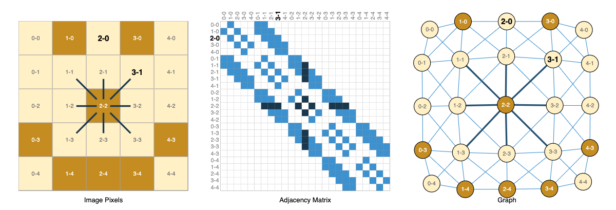
GCN (Graph Convolutional Networks) 은 그래프 구조 데이터에서 노드(Node)와 엣지(Edge) 정보를 활용하여 특징(Feature)을 학습하는 딥러닝 모델임. 이미지 처리에 주로 사용되는 CNN(Convolutional Neural Networks)의 합성곱 연산을 그래프 데이터로 확장한 개념으로, 이웃 노드들의 정보를 집계(Aggregate)하여 현재 노드의 표현(Representation)을 업데이트하는 방식을 사용함.

등장배경​

• 비유클리드 데이터 처리의 한계: 기존의 CNN은 이미지나 텍스트와 같이 격자(Grid) 구조를 가진 유클리드 데이터(Euclidean Data)에서 뛰어난 성능을 보였으나, 소셜 네트워크, 분자 구조, 웹 링크 등 불규칙한 관계를 가진 **비유클리드 데이터(Non-Euclidean Data)**를 처리하는 데에는 한계가 존재함.
• 관계성 정보의 중요성: 데이터 자체의 속성뿐만 아니라 데이터 간의 **연결 관계(Structure)**가 중요한 정보를 담고 있는 경우가 많아, 이를 효과적으로 학습할 수 있는 모델이 필요해짐.

유형​

• Node Classification: 노드의 속성이나 레이블을 예측하는 작업
• Graph Classification: 그래프 전체의 속성이나 레이블을 예측하는 작업
• Node Clustering: 노드들을 유사한 특성을 가진 그룹으로 묶는 작업
• Link Prediction: 그래프 내에서 존재하지 않는 엣지를 예측하는 작업
• Influence Maximization: 그래프 내에서 영향력을 극대화할 수 있는 노드를 찾는 작업

구성도​

GCN은 기본적으로 입력된 그래프 데이터에 대해 여러 번의 그래프 합성곱 연산(Graph Convolution)과 활성화 함수(Activation Function)를 거쳐 최종적으로 노드 분류나 링크 예측 등의 작업을 수행함.

1. Input Layer: 노드의 특징 행렬($X$)과 인접 행렬($A$)을 입력받음.
2. Hidden Layers (Graph Convolution): 각 노드는 이웃 노드의 정보를 모아 자신의 정보를 갱신함. (Message Passing)
3. Activation Function: 비선형성(Non-linearity)을 추가하기 위해 ReLU 등을 사용함.
4. Output Layer: 최종적으로 학습된 노드 임베딩을 사용하여 분류(Classification)나 회귀(Regression) 등의 태스크를 수행함.

GCN의 유형​

GCN은 접근 방식에 따라 크게 두 가지 유형으로 분류됨.

1. 스펙트럼 기반 (Spectral-based GCNs)

   • 그래프 신호 처리 이론에 기반하여, 그래프 라플라시안(Graph Laplacian)과 푸리에 변환(Fourier Transform)을 이용해 스펙트럼 도메인에서 합성곱을 수행함.
   • 특징: 이론적 토대가 탄탄하지만, 그래프 전체 구조에 의존적이어서 구조가 바뀌면 재학습이 필요하며 계산 복잡도가 높음.
   • 대표 모델: ChebNet (Chebyshev 다항식 근사), GCN (Kipf & Welling의 1차 근사).

2. 공간 기반 (Spatial-based GCNs)

   • 노드의 공간적 이웃 관계를 기반으로 정보를 직접 집계(Aggregation)하는 방식. CNN 필터가 픽셀 위를 이동하는 것과 유사함.
   • 특징: 직관적이며 계산 효율성이 높고, 거대 그래프나 유동적인 그래프에도 적용하기 용이함.
   • 대표 모델: GraphSAGE (이웃 샘플링), GAT (Attention 가중치).

구성요소​

작동 원리​

GCN의 핵심 작동 원리는 메시지 패싱(Message Passing) 으로, 이웃 노드의 정보를 수집하고 가중치를 적용하여 자신의 상태를 업데이트하는 과정임.

1. 수학적 정의​

가장 널리 쓰이는 Kipf & Welling의 GCN 레이어 갱신 규칙은 다음과 같음.

• $H^{(l)}$: $l$번째 층의 노드 특징 행렬 ($N \times D$).
• $\tilde{A}$: 정규화된 인접 행렬 (Normalized Adjacency Matrix).
  • 보통 $\tilde{A} = D^{-\frac{1}{2}}\hat{A}D^{-\frac{1}{2}}$로 정의 ($\hat{A} = A + I$, $I$는 자기 자신을 포함하기 위한 단위 행렬).
• $W^{(l)}$: 학습 가능한 가중치 행렬 ($D \times F$).
• $\sigma$: 활성화 함수 (ReLU 등).

2. 정규화​

단순히 인접 행렬 $A$를 곱하면 연결이 많은 노드(Hub)의 값이 폭발적으로 커지거나, 적은 노드는 소실될 수 있음. 이를 방지하기 위해 차수(Degree) $D$를 이용해 정규화($D^{-\frac{1}{2}}AD^{-\frac{1}{2}}$)를 수행하여 수치적 안정성을 확보함.

3. 구현 예시​

import numpy as np

def graph_convolutional_layer(A, X, W):
    # A: Adjacency matrix, X: Input features, W: Weights
    
    # 1. Self-loop 추가 (자기 자신의 정보도 포함하기 위함)
    I = np.eye(A.shape[0])
    A_hat = A + I
    
    # 2. 차수 행렬 계산 및 정규화 (Normalization)
    D = np.sum(A_hat, axis=0)
    D_inv_sqrt = np.power(D, -0.5)
    D_inv_sqrt[np.isinf(D_inv_sqrt)] = 0.
    D_mat_inv_sqrt = np.diag(D_inv_sqrt)
    
    # A_norm = D^-0.5 * A_hat * D^-0.5
    A_norm = np.dot(np.dot(D_mat_inv_sqrt, A_hat), D_mat_inv_sqrt)
    
    # 3. 집계 및 변환 (Aggregation & Transformation)
    output = np.dot(A_norm, X)  # 이웃 정보 집계
    output = np.dot(output, W)  # 가중치 변환
    
    return output

CNN과의 비교​

주요 변형 모델 (Variants)​

• GraphSAGE: 모든 이웃을 사용하는 GCN의 계산 비용 문제를 해결하기 위해, 고정된 수의 이웃을 **샘플링(Sampling)**하여 집계함.
• GAT (Graph Attention Networks): 모든 이웃에 동일한 중요도를 부여하는 대신, 어텐션(Attention) 메커니즘을 적용하여 더 중요한 이웃의 정보에 높은 가중치를 부여함.
• ChebNet: 스펙트럼 기반 방식을 효율화하기 위해 Chebyshev 다항식을 사용하여 필터를 근사함.
• GIN (Graph Isomorphism Network): 그래프 동형성(Isomorphism)을 구분할 수 있을 정도로 강력한 표현력을 갖도록 설계됨.

장단점​

활용방안​

• 소셜 네트워크 분석 (Social Network Analysis): 친구 추천(Facebook), 커뮤니티 탐지, 가짜 뉴스 전파 경로 분석.
• 생물정보학 및 화학 (Bioinformatics & Chemistry): 신약 개발을 위한 분자 구조 분석(Drug Discovery), 단백질 상호작용 예측.
• 추천 시스템 (Recommender Systems): 사용자(User)와 아이템(Item) 간의 상호작용 그래프를 분석하여 정교한 추천 제공 (Pinterest 등).
• 지식 그래프 (Knowledge Graph): 개체 간의 복잡한 관계를 추론하고 질의응답 시스템 고도화(Google).
• 컴퓨터 비전 (Computer Vision): 이미지 내 객체 간의 관계를 그래프로 모델링하여 장면(Scene) 이해.

최근 연구 동향​

1. GNN과 LLM의 융합 (GNN-LLM Convergence): GCN 모델 자체의 개선을 넘어, GraphRAG와 같이 지식 그래프를 인코딩하여 LLM의 추론을 돕거나 상호보완하는 연구가 주류를 이룸.
2. 그래프 파운데이션 모델 (Graph Foundation Models): 특정 태스크에 국한되지 않고, 다양한 그래프 데이터에 범용적으로 적용 가능한 대규모 사전 학습 모델(Pre-trained Models) 개발이 가속화됨.
3. Graph Transformers: 기존 메시지 패싱(Message Passing) 방식의 한계를 넘어서기 위해, 트랜스포머(Transformer) 아키텍처를 그래프 도메인에 최적화하여 적용하는 연구 활발.
4. 생성형 GNN (Generative GNNs): 신약 개발이나 소재 설계 등에서 원하는 속성을 가진 새로운 그래프 구조를 생성하는 확산 모델(Diffusion Models) 기반 연구 증가.
5. 설명 가능성 및 신뢰성 (Explainability & Trustworthiness): 금융이나 의료 등 민감한 분야의 도입 확대로 인해, 모델의 예측 근거를 제시하고 견고성(Robustness)을 확보하는 기술이 필수적임.

Ref​

• A Gentle Introduction to Graph Neural Networks

Vocabulary & Expressions​

• get to:
  • access 가능 지점에 도착
  • 감정적으로 도달함
  • 물리적 도착
  • 기회지점에 도착
  • get (이동/변화) + to (목표지점)

Vocabulary & Expressions​

Summary​

• This study reformulates Drone-BS 3D deployment as a SINR-based coverage probability optimization problem rather than a distance- or area-based one.
• By jointly considering LOS/NLOS propagation, altitude-dependent SINR behavior, and system constraints, the deployment problem is formulated as an NP-hard MINLP.
• A meta-heuristic optimizer (GWO) is used as a practical solver, demonstrating that high coverage can be achieved with a minimal number of Drone-BSs.

Introduction​

Background​

• In 5G networks, Drone-BSs (UAV-BSs) have attracted significant attention as a promising solution to enhance coverage and capacity in dense urban environments.
• Although the use of the mmWave band enables high data rates, determining the optimal 3D deployment (horizontal location and altitude) of Drone-BSs has emerged as a critical challenge.

Limitations of Existing Studies​

• Assumption of fixed Drone-BS altitude
• Reliance on heuristic-based approaches
• Consideration of limited system constraints

Objective of This Study​

• This study aims to derive an optimal Drone-BS deployment strategy by combining
• SINR-based downlink coverage probability analysis and
• a meta-heuristic optimization algorithm, namely the Grey Wolf Optimizer (GWO).

Methods​

System Model​

• Users (N) and Drone-BSs (M) are randomly distributed in an urban environment.
• A mmWave path loss model considering LOS and NLOS propagation conditions is applied.
• A predefined SINR threshold is used as the Quality-of-Service (QoS) criterion.

Coverage Probability Analysis​

• The probability that SINR exceeds a predefined threshold is derived based on stochastic geometry.
• Shadow fading is modeled as a Gaussian random variable.
• The downlink coverage probability is expressed using a Q-function formulation.

Optimization Problem Formulation​

• Objective function
  • Maximize the number of covered users.
• Constraints
  • Minimum number of deployed Drone-BSs
  • Drone-BS altitude limits
  • Total available bandwidth constraint
• The problem is formulated as a Mixed Integer Non-Linear Programming (MINLP) problem and is NP-hard.

Solution Approach​

• The Grey Wolf Optimizer (GWO) is employed to search for the optimal 3D locations (x, y, h) of Drone-BSs.

Results​

Simulation Setup​

• Area size: 2 × 2 km²
• Number of users: 200
• Maximum number of Drone-BSs: 10
• Carrier frequency: 28 GHz

Key Findings​

• The downlink coverage probability increases as the Drone-BS altitude increases.
• A coverage probability of approximately 0.76–0.82 can be achieved with only five Drone-BSs.
• Reducing the number of Drone-BSs leads to uncovered regions.
• Increasing the number of Drone-BSs may result in higher inter-cell interference.

Discussion​

Performance Analysis​

• The GWO-based deployment achieves high coverage performance while minimizing the number of Drone-BSs.
• Increasing altitude improves coverage but introduces a trade-off in terms of reduced energy efficiency.

Limitations and Future Work​

• The proposed approach does not consider blockage effects or handover and coverage overlap issues.
• These aspects are identified as important directions for future research.

Terminology​

• Drone-BS: Drone Base Station
• GWO: Grey Wolf Optimizer, a nature-inspired optimization algorithm based on the social hierarchy and hunting behavior of grey wolves.
• LOS: Line of Sight, a direct path between transmitter and receiver without obstructions.
• MINLP: Mixed Integer Non-Linear Programming, an optimization problem involving both integer and continuous variables with non-linear relationships.
• NLOS: Non-Line of Sight, a path between transmitter and receiver that is obstructed.
• SINR: Signal to Interference plus Noise Ratio, a measure of signal quality.
• UVA-BS: Unmanned Aerial Vehicle Base Station

Ref​

• Ouamri, M. A., Oteşteanu, M.-E., Barb, G., & Gueguen, C. (2022). Coverage Analysis and Efficient Placement of Drone-BSs in 5G Networks. The 1st International Conference on Computational Engineering and Intelligent Systems, 18. https://doi.org/10.3390/engproc2022014018

Summary​

• Model performance in 5G coverage prediction is primarily determined by the alignment between data characteristics, feature design, and model inductive bias, rather than by model complexity alone.
• Using real-world 5G NR drive-test data with physics-informed numerical features, this study demonstrates that Random Forest can achieve SOTA performance, outperforming more complex models such as XGBoost and deep neural networks.
• The results highlight the continued importance of domain-informed feature engineering and show that deep learning becomes advantageous only when the data representation and scale justify its use.

Introduction​

• Coverage prediction in 5G networks is a core component of network planning, optimization, and resource allocation.
• Conventional propagation and path loss models are limited in their ability to accurately capture the complexity of dense urban environments and the unique characteristics of 5G systems.
• Machine Learning and Deep Learning have emerged as promising alternatives, as they can model complex non-linear relationships across multiple parameters.
• However, prior studies typically suffer from several limitations:
  • Most focus on 4G networks or rely on a limited set of input features.
  • Comparisons across a wide range of algorithms are often insufficient.
  • Systematic analyses of feature importance are largely lacking.

The objectives of this study are to:

• Conduct a comprehensive comparison of multiple ML and DL algorithms using a unified dataset.
• Identify dominant feature parameters that significantly influence 5G coverage prediction.
• Demonstrate performance improvements over previously reported methods.

Methods​

Data Collection​

• Real-world 5G NR drive test measurements conducted in Bandung, Indonesia (Batununggal area).
• Approximately 1,500 SS-RSRP samples collected.
• Deployment includes 10 gNodeBs, each configured with three sectors.
• Measurement vehicle speed maintained below 30 km/h to minimize fast fading effects.

Input Features (10 Total)​

• 2D Distance between Transmitter and Receiver
• Frequency
• Transmitter Tilt Angle
• Transmitter Azimuth Angle
• Altitude
• Elevation Angle
• Azimuth Offset Angle
• Tilting Offset Angle
• Horizontal Distance of Receiver from Transmitter Antenna Boresight
• Vertical Distance of Receiver from Transmitter Antenna Boresight

Algorithms​

Machine Learning (Classification-based):

• Logistic Regression
• K-Nearest Neighbors (KNN)
• Naive Bayes
• Random Forest
• Support Vector Machine (SVM)
• XGBoost
• LightGBM
• AdaBoost
• Bayesian Network Classifier

Deep Learning:

• Multi-Layer Perceptron (MLP)
• Long Short-Term Memory (LSTM)
• Convolutional Neural Network (CNN)

Training and Validation​

• Experiments conducted using Google Colab.
• 10-fold cross-validation applied for all models.
• Hyperparameter optimization performed only on the best-performing models.

Evaluation Metrics​

• Regression Metrics: RMSE, MAE, R²
• Classification Metrics: Accuracy, Precision, Recall, F1-score

Results​

Machine Learning​

Random Forest:

• RMSE = 1.14 dB
• MAE = 0.12
• R² = 0.97
• Accuracy / Precision / Recall / F1-score ≈ 98.4%

Deep Learning​

Convolutional Neural Network (CNN):

• RMSE = 0.289

• MAE = 0.289

• R² = 0.78

• Accuracy = 75%

• Precision = 85.6%

• Recall = 87.8%

• F1-score = 89.9%

• MLP and LSTM exhibit inferior performance compared to CNN.

Feature Importance​

• The 2D Transmitter–Receiver Distance is identified as the most dominant feature across all algorithms.
• Incorporating horizontal and vertical distances from the antenna boresight significantly improves prediction accuracy.

Comparison with Previous Studies​

• Both Random Forest and CNN achieve lower RMSE values compared to prior studies.
• Random Forest, in particular, demonstrates state-of-the-art performance relative to existing 4G and 5G coverage prediction research.

Discussion​

• Random Forest
  • Highly effective for small-to-medium-sized datasets with numerical features.
  • Offers strong interpretability and robust performance stability.
• Convolutional Neural Network
  • Well-suited for grid-based or spatial data representations.
  • Shows greater potential when image-based or satellite-derived features are incorporated.
  • In this study, CNN was applied by transforming numerical features into a matrix-like structure.
• The results empirically demonstrate that feature design and selection can be more critical than the choice of learning algorithm itself.

현대자동차에 합류하기 전, 인사팀에서는 진급이 거의 확정적인 것처럼 이야기했었다. 하지만 막상 들어와 보니 실상은 많이 달랐다. 나름 열심히 했다고 생각했지만, 작년 첫 고과에서 나는 1월 입사자라는 이유로 평가 대상에서 제외되었고 그 때문에 리스트에도 오르지 못한 것이 아닐까 싶다.

규칙이라면 따라야겠지만, 인사와 내부 사정이 다른 것에 실망스러웠다. 비슷한 연차의 동료들 역시 각자 나름의 불만을 안고 출발했던 것 같다. 바꿀 수 없는 것보다는 바꿀 수 있는 것에 집중하자는 생각으로, 나는 다른 일들에 더 많은 시간을 쓰게 되었다.

1분기는 목표가 사라진 채로 거의 의욕 없이 흘려보냈다. 그 전까지는 대학원 시험을 잘 치르는 것이 가장 큰 목표였는데, 결과 발표가 계속 미뤄지면서 마음이 더 힘들어졌다. 여러 번 연기되었던 결과는 4월 초에야 나왔고, 낙방이었다. 그 원인이 GPA인지, 시험 결과인지, SOP인지, 영어 성적인지 무엇이 부족했는지 궁금해 문의했지만 구체적인 답을 듣지는 못했다. 대신 아래와 같은 답변을 받을 수 있었다.

We regret to inform you that your application in this admission cycle was not successful. Please understand that admission into the Master of Science in Machine Learning is very competitive and takes into account a large number of criteria. Due to restrictions on the number of places, we unfortunately have to decline a large number of strong applications. Although this final decision may be disappointing, we are confident that, given your credentials, many other opportunities will open up for you.

"Strong applications"라는 표현에 그나마 위안을 얻었던 것 같다. 하지만 다시 같은 꿈을 꾸기에는 아이엘츠 성적 만료가 코앞이었고, 재도전은 현실적으로 어려워 보였다. 한정된 시간 안에서 무엇을 해야 할지 고민하던 중, 예전부터 와이프가 추천해주던 유학원과 박람회가 떠올랐다.

코엑스에서 주기적으로 열리는 유학·해외취업·이민 박람회를 찾아보고, 별다른 기대 없이 무작정 찾아갔다. 영국 석사는 1.5년 코스였지만, 아이엘츠의 영국 전용 버전이 신설되면서 기존 성적을 사용할 수 없었다. 그 대안으로 호주가 눈에 들어왔다. 아랍에미리트의 다른 대학원도 가능성은 있었지만, 예전부터 시드니에서 살아보고 싶다고 말하던 와이프의 영향으로 호주 대학원을 목표로 삼게 되었다.

박람회에서 연결된 유학원은 생각보다 체계적이지 않았고, 진행 과정도 만족스럽지는 않았다. 그럼에도 불구하고 인공지능으로 급변하는 소프트웨어 엔지니어 정의와 미래를 대비해야 한다는 생각, 그리고 물리 AI 시대가 오기 전에 관련 기업으로 이직하거나 연구로 방향을 틀어야 한다는 판단은 분명했다. 그렇게 인공지능 석사를 목표로 상담을 이어갔다. 아이엘츠 성적과, 자금, 경력, 그리고 의지도 있었기에 과정은 비교적 빠르게 진행되었다. 그 무렵 퇴사 의사를 밝혔고, 멋진 동료들로부터 불확실한 앞길에 대해 따뜻한 덕담을 받을 수 있었다는 점이 참 감사했다.

집을 팔고, 가진 것들을 정리한 뒤, 캐리어 두 개만 들고 7월 13일 호주에 도착했다. 예상보다 훨씬 쌀쌀했던 호주의 겨울에 적응하는 일은 쉽지 않았다. 한국에서는 영어를 꽤 한다고 생각했지만, 내가 익숙했던 것은 정제된 영어였다는 걸 곧 깨달았다. 현지인들의 영어와 영어를 세컨드 랭기지로 사용하는 친구들의 영어는 완전히 달랐다.

게다가 한국어로도 아카데믹 레포트에 익숙하지 않은 상태에서, 짧은 시간 안에 영어 레퍼런스를 포함한 IMRD 포맷의 리포트를 작성하는 일은 정말 버거웠다. "이만큼 돈을 쓰는데 석사 학위쯤은 그냥 살 수 있는 거 아니야?"라고 생각했던 과거의 내가 부끄러워졌다. ChatGPT조차 없던 시절에 해외 석박을 마친 선배님들이 새삼 대단하게 느껴졌다. 몇몇 뛰어난 20대 글로벌 인재들을 보며, 그들의 10년 뒤 모습이 궁금해지기도 했다.

수업과 과제, 시험에 적응해 가는 시간 속에서, 와이프가 잠깐씩 지구 반대편으로 와줄 때마다 마음의 여유를 얻을 수 있었다. 그렇게 New South Wales 주에서의 혼인신고까지 마무리하며, 1학기를 High Distinction으로 잘 끝낼 수 있었다. 마지막 달에는 멋진 슈퍼바이저 밑에서 재미있는 연구를 같이할 기회도 얻었다. 시간이 날 때마다 해보고 싶었던 코드 템플릿화와 프롬프트화 역시 그 마지막 달에 시도해볼 수 있었다.

내년에는 어떤 회고를 쓰게 될까. 벌써부터 기대가 된다.

shadcn/ui(Vaul)를 사용하여 모바일 웹을 개발하던 중, iOS Safari에서 Drawer 내부의 Dialog를 호출할 때 발생하는 스크롤 충돌 버그를 해결했다.

문제 상황​

모바일 뷰에서 '더보기' Drawer를 열고 내부 메뉴를 클릭하여 '공유하기' Dialog를 띄우는 기능이었다.

1. Drawer Open: 스크롤이 있는 페이지에서 Drawer를 연다.
2. Interaction: 메뉴 클릭 시 Drawer가 닫히고 Dialog가 열린다.
3. Bug: 이 전환 과정에서 배경 스크롤이 최상단으로 초기화(Jump to Top) 되거나, 화면이 고정되어 먹통이 된다.

원인 분석: Scroll Lock Race Condition​

• Vaul(Drawer)도 Radix Dialog 기반이라, Drawer close 직후 Dialog open이 같은 프레임/틱에서 일어나면 중첩된 overlay의 스크롤 락/바디 스타일 변경이 겹치며 iOS Safari에서 스크롤 복원/점프가 발생할 수 있다

해결 방법​

1. Timing (실행 시점 분리)​

onClose나 클릭 핸들러에서 즉시 Dialog를 띄우지 않고, onAnimationEnd 이벤트를 활용하여 Drawer의 정리가 완전히 끝난 후 Dialog를 호출해야 한다.

<Drawer
  onAnimationEnd={(open) => {
    // Drawer가 완전히 닫힌 후(!open) 실행
    if (!open) {
      setDialogOpen(true);
    }
  }}
>

2. Configuration (iOS 호환성 옵션)​

Vaul 컴포넌트에 다음 옵션을 추가하여 Safari의 불완전한 스타일 재계산을 방지한다.

<Drawer
  disablePreventScroll={true}
  repositionInputs={false}
  shouldScaleBackground={false}
>

• disablePreventScroll={true}
  • Vaul이 body에 강제로 스크롤 락 스타일을 적용하지 않도록 한다
  • iOS에서 발생하는 스크롤 점프 현상을 완화
  • 단, Drawer가 열려 있는 동안 배경 스크롤이 허용될 수 있음
• repositionInputs={false}
  • 가상 키보드 대응을 위한 viewport 재배치 로직 비활성화
  • iOS Safari에서 input + 모달 조합 시 발생하는 레이아웃 충돌 방지
• shouldScaleBackground={false}
  • Drawer 오픈 시 배경을 scale 처리하지 않음
  • 불필요한 body 스타일 변경을 줄여 안정성 확보

이 옵션들은 완전한 해결책이라기보다는 iOS Safari 환경에서의 리스크를 줄이기 위한 방어설정에 가깝긴하다.

Ref​

• Github Issue: Vaul Drawer iOS Scroll Bug

OpenQASM 2.0​

오픈캐즘

OPENQASM 2.0; // 언어 버전 선언

qreg q[1]; // 큐비트 레지스터 q를 선언 (큐비트 1개, 초기 상태 |0⟩)
creg c[1]; // 고전 비트 레지스터 c를 선언 (측정 결과 저장용)

h q[0]; // Hadamard 게이트 적용: |0⟩ → (|0⟩ + |1⟩) / √2

measure q[0] -> c[0]; // q[0]을 측정하고 결과(0 또는 1)를 c[0]에 저장

OPENQASM 2.0;

qreg q[10]; // ∣0000000000⟩
creg c[10];

// x 게이트를 사용하여 처음 세 큐비트를 ∣1⟩ 상태로 변경
x q[0]; ∣1000000000⟩
x q[1]; ∣1100000000⟩
x q[2]; ∣1110000000⟩

measure q[0] -> c[0]; // 1
measure q[1] -> c[1]; // 1
measure q[2] -> c[2]; // 1

Linear Algebra​

Vectors​

• In quantum computing, vectors represent quantum states.
• A 2-dimensional vactor can be written as:
• $|\psi\rangle = \begin{pmatrix} \psi_0 \\ \psi_1 \end{pmatrix}$

Computational Basis​

$|0\rangle = \begin{pmatrix} 1 \\ 0 \end{pmatrix}, \quad |1\rangle = \begin{pmatrix} 0 \\ 1 \end{pmatrix}$

• $|\psi\rangle$ is a linear combination of basis states as follows:
• $|\psi\rangle = \psi_0|0\rangle + \psi_1|1\rangle = \begin{pmatrix} \psi_0 \\ \psi_1 \end{pmatrix}$

Indentity Matrix​

• $\mathbb I \psi\rangle = \begin{bmatrix} \psi_0 \\ \psi_1 \end{bmatrix}$
• $\mathbb I^2 = \begin{bmatrix} 1 & 0 \\ 0 & 1 \end{bmatrix}$

Conjugate Transpose​

• Bra: $|\psi\rangle^\dagger = \begin{pmatrix} \psi_0 \\ \psi_1 \end{pmatrix}^\dagger = \begin{pmatrix} \overline{\psi_0} & \overline{\psi_1} \end{pmatrix} = \langle \psi|$
  • $\langle \psi| := |\psi\rangle^\dagger$
  • ket: $|\psi\rangle$
  • bra: $\langle \psi|$
  • bra + ket: dot product $\langle \phi|\psi\rangle$
• Dagger: $A = \begin{bmatrix} a & b \\ c & d \end{bmatrix} \implies A^\dagger = \begin{bmatrix} \overline{a} & \overline{c} \\ \overline{b} & \overline{d} \end{bmatrix}$

psi_dagger = psi.conjugate().T
psi_dagger = psi.conjugate().transpose()
psi_dagger = psi.H

• $(\alpha A)\dagger = \overline\alpha A^\dagger$
• $(A^\dagger)^\dagger = A$
• $(A + B)^\dagger = A^\dagger + B^\dagger$
• $(AB)^\dagger = B^\dagger A^\dagger$

Hermitian​

• A matrix is equal to its conjugate transpose.
• $H = H^\dagger$

A_dagger = A.H
AA_dagger = A * A_dagger
# (AA†)†=AA†?
is_hermitian = AA_dagger.is_hermitian

Unitary​

• A matrix whose conjugate transpose is also its inverse.
• $U^\dagger U = U U^\dagger = \mathbb I$
• $U = \begin{pmatrix} \cos\theta & \sin\theta \\ -\sin\theta & \cos\theta \end{pmatrix}$

U = Matrix([
  [cos(theta), sin(theta)], 
  [-sin(theta), cos(theta)]
])

U_dagger = U.H
U_dagger_U = trigsimp(U_dagger * U)

is_unitary = U_dagger_U == I

Inner Product​

• $\langle \psi|\phi\rangle = \begin{pmatrix} \overline{\psi_0} & \overline{\psi_1} \end{pmatrix} \begin{pmatrix} \phi_0 \\ \phi_1 \end{pmatrix} = \overline{\psi_0}\phi_0 + \overline{\psi_1}\phi_1$
• $|\langle \psi|\phi\rangle|^2 = \langle \psi|\phi\rangle \langle \phi|\psi\rangle$
• $|\langle\psi|\phi\rangle| = |\langle\phi|\psi\rangle|$

Orthogonality​

• $|0\rangle = \begin{pmatrix} 1 \\ 0 \end{pmatrix}, \quad |1\rangle = \begin{pmatrix} 0 \\ 1 \end{pmatrix}$
  • orthonormal basis
• $\langle 0 | 1 \rangle = \begin{pmatrix} 1 & 0 \end{pmatrix} \begin{pmatrix} 0 \\ 1 \end{pmatrix} = 0$
  • $\langle 1 | 0 \rangle = 0$
• $\langle 0 | 0 \rangle = \begin{pmatrix} 1 & 0 \end{pmatrix} \begin{pmatrix} 1 \\ 0 \end{pmatrix} = 1$
  • $\langle 1 | 1 \rangle = 1$

$\langle \psi|\phi\rangle = \overline{\psi_0}\phi_0 + \overline{\psi_1}\phi_1$

• $|\psi\rangle = \psi_0|0\rangle + \psi_1|1\rangle, \quad |\phi\rangle = \phi_0|0\rangle + \phi_1|1\rangle$
• $\langle \psi| = \overline{\psi_0}\langle 0| + \overline{\psi_1}\langle 1|$
• $\langle \psi|\phi\rangle = \overline{\psi_0}\phi_0\langle 0|0\rangle + \overline{\psi_0}\phi_1\langle 0|1\rangle + \overline{\psi_1}\phi_0\langle 1|0\rangle + \overline{\psi_1}\phi_1\langle 1|1\rangle$
• $\langle 0|1\rangle = 0, \quad \langle 1|0\rangle = 0$

Magnitude​

$\|\psi\rangle\|^2 = |\psi_0|^2 + |\psi_1|^2$

• $\|\psi\rangle\| = \sqrt{\langle \psi|\psi\rangle} = \sqrt{|\psi_0|^2 + |\psi_1|^2}$
• $\| |\psi\rangle\|^2 = \langle \psi|\psi\rangle$
  • $\langle \psi|\psi\rangle = \overline{\psi_0}\psi_0 + \overline{\psi_1}\psi_1 = |\psi_0|^2 + |\psi_1|^2$

Outer product​

• $|\psi\rangle\langle\phi| = (\psi_0 | 0\rangle + \psi_1 |1\rangle)(\overline{\phi_0}\langle 0| + \overline{\phi_1}\langle 1|) \\ \quad =\psi_0\overline{\phi_0}|0\rangle\langle 0| + \psi_0\overline{\phi_1}|0\rangle\langle 1| + \psi_1\overline{\phi_0}|1\rangle\langle 0| + \psi_1\overline{\phi_1}|1\rangle\langle 1|$
• $|\psi\rangle\langle\phi| = \begin{pmatrix} \psi_0 \\ \psi_1 \end{pmatrix} \begin{pmatrix} \overline{\phi_0} & \overline{\phi_1} \end{pmatrix} = \begin{pmatrix} \psi_0\overline{\phi_0} & \psi_0\overline{\phi_1} \\ \psi_1\overline{\phi_0} & \psi_1\overline{\phi_1} \end{pmatrix}$
• $|0\rangle = \begin{pmatrix} 1 \\ 0 \end{pmatrix}, \quad |1\rangle = \begin{pmatrix} 0 & 1 \end{pmatrix}$
• $|0\rangle\langle 0| = \begin{pmatrix} 1 \\ 0 \end{pmatrix} \begin{pmatrix} 0 & 1 \end{pmatrix} = \begin{pmatrix} 0 & 1 \\ 0 & 0 \end{pmatrix}$
• $A = \begin{pmatrix} a_{00} & a_{0 1} \\ a_{1 0} & a_{1 1} \end{pmatrix} \\ \quad = a_{00}|0\rangle\langle 0| + a_{01}|0\rangle\langle 1| + a_{10}|1\rangle\langle 0| + a_{11}|1\rangle\langle 1|$

Tensor Product​

• $|\psi\rangle \otimes |\phi\rangle = \begin{pmatrix} \psi_0 \\ \psi_1 \end{pmatrix} \otimes \begin{pmatrix} \phi_0 \\ \phi_1 \end{pmatrix} = \begin{pmatrix} \psi_0\phi_0 \\ \psi_0\phi_1 \\ \psi_1\phi_0 \\ \psi_1\phi_1 \end{pmatrix}$
• $|\psi\rangle \otimes |\phi\rangle \equiv |\psi\rangle|\phi\rangle \equiv |\psi\phi\rangle$
• $A \otimes B = \begin{pmatrix} a_{00}B & a_{01}B \\ a_{10}B & a_{11}B \end{pmatrix}$
• $|0\rangle \langle 1| \otimes |1\rangle \langle 0| = \begin{pmatrix} 0 & 1 \\ 0 & 0 \end{pmatrix} \otimes \begin{pmatrix} 0 & 0 \\ 1 & 0 \end{pmatrix}$
• $|0\rangle \langle 1| \otimes |1\rangle \langle 0| = \begin{pmatrix} 0\begin{pmatrix} 0 & 0 \\ 1 & 0 \end{pmatrix} & 1\begin{pmatrix} 0 & 0 \\ 1 & 0 \end{pmatrix} \\ 0\begin{pmatrix} 0 & 0 \\ 1 & 0 \end{pmatrix} & 0\begin{pmatrix} 0 & 0 \\ 1 & 0 \end{pmatrix} \end{pmatrix} = \begin{pmatrix} 0 & 0 & 0 & 0 \\ 0 & 0 & 1 & 0 \\ 0 & 0 & 0 & 0 \\ 0 & 0 & 0 & 0 \end{pmatrix}$
• $|0\rangle \langle 1| \otimes |1\rangle \langle 0| \equiv (|0\rangle \otimes |1\rangle)(\langle 1| \otimes \langle 0|) \\ \quad \equiv |0\rangle|1\rangle \langle 0|\langle 1| \\ \quad \equiv |01\rangle \langle 10|$
  • $ket \otimes ket, \quad bra \otimes bra$

Qubit​

$|\psi\rangle = \alpha|0\rangle + \beta|1\rangle$

• where $\alpha, \beta$ are complex numbers satisfying $|\alpha|^2 + |\beta|^2 = 1$.
• phase factor: $e^{i\phi}$, turn the state by angle $\phi$ in the complex plane, but does not affect measurement probabilities.
  • $|e^{i\phi}| = 1$

One-Qubit Gates​

Identity Gate​

$\mathbb{I} = \begin{pmatrix} 1 & 0 \\ 0 & 1 \end{pmatrix}$

Pauli-X Gate​

$X = \begin{pmatrix} 0 & 1 \\ 1 & 0 \end{pmatrix}$

• NOT gate

Pauli-Y Gate​

$Y = \begin{pmatrix} 0 & -i \\ i & 0 \end{pmatrix}$

Pauli-Z Gate​

$Z = \begin{pmatrix} 1 & 0 \\ 0 & -1 \end{pmatrix}$

Hadamard Gate​

$H = \frac{1}{\sqrt{2}} \begin{pmatrix} 1 & 1 \\ 1 & -1 \end{pmatrix}$

Rotation Gate​

$R(\theta) = \begin{pmatrix} \cos{\theta} & \sin{\theta} \\ -\sin{\theta} & \cos{\theta} \end{pmatrix}$

The Bloch Sphere​

$|\psi\rangle = \cos(\theta) |0\rangle + e^{i\phi}\sin(\theta)|1\rangle$

• where $0 \leq \theta \leq \pi$ and $0 \leq \phi < 2\pi$.
• $\theta$: the polar (or colatitude) angle, measured from the "north pole" of the sphere.
  • polar angle: 편각
• $\phi$: the azimuthal (or longitude) angle around the equator.
  • azimuthal angle: 방위각

Two-Qubit Gates​

CNOT Gate​

Controlled-NOT or CX gate

$CNOT = \begin{pmatrix} 1 & 0 & 0 & 0 \\ 0 & 1 & 0 & 0 \\ 0 & 0 & 0 & 1 \\ 0 & 0 & 1 & 0 \end{pmatrix}$

• CNOT gate flips the second qubit (target) if the first qubit (control) is $|1\rangle$.

SWAP Gate​

$SWAP = \begin{pmatrix} 1 & 0 & 0 & 0 \\ 0 & 0 & 1 & 0 \\ 0 & 1 & 0 & 0 \\ 0 & 0 & 0 & 1 \end{pmatrix}$

• SWAP gate exchanges the states of the two qubits.

Controlled-Z Gate​

$CZ = \begin{pmatrix} 1 & 0 & 0 & 0 \\ 0 & 1 & 0 & 0 \\ 0 & 0 & 1 & 0 \\ 0 & 0 & 0 & -1 \end{pmatrix}$

• CZ gate applies a Z gate to the second qubit if the first qubit is in state $|1\rangle$.

Bases​

• Computational Basis: $\{|0\rangle, |1\rangle\}$
• two qubits: $\{|00\rangle, |01\rangle, |10\rangle, |11\rangle\}$
• three qubits: $\{|000\rangle, |001\rangle, |010\rangle, |011\rangle, |100\rangle, |101\rangle, |110\rangle, |111\rangle\}$

Rule of Thumb​

What starts on the left of the tensor product stays on the left.

• $|\psi\rangle \otimes |\phi\rangle \equiv |\psi\rangle|\phi\rangle \equiv |\psi\phi\rangle$
• $(|\psi\rangle \otimes |\phi\rangle)^* = \langle\psi| \otimes \langle\phi|$
• $(\alpha |\psi\rangle + \beta |\phi\rangle) \otimes |\omega\rangle = \alpha|\psi\rangle \otimes |\omega\rangle + \beta |\phi\rangle \otimes | \omega\rangle$
• $(\langle\psi| \otimes \langle\phi|)(|\omega\rangle \otimes |\eta\rangle) = \langle\psi|\omega\rangle \cdot \langle\phi|\eta\rangle)$
• $(A + B) \otimes C = A \otimes C + B \otimes C$
• $A \otimes (B + C) = A \otimes B + A \otimes C$
• $(A \otimes B)(C \otimes D) = (AC) \otimes (BD)$
• $(A \otimes B)^* = A^* \otimes B^*$

Entanglement​

• $|\Psi\rangle = \alpha_{00} |00\rangle + \alpha_{01} |01\rangle + \alpha_{10} |10\rangle + \alpha_{11} |11\rangle$
  • where $\|\Psi\rangle\|^2 = 1$
• If the state is not separable, it is entangled.
• A state is separable if it can be written as a tensor product of two individual qubit state.
• $|\Psi\rangle = \frac{1}{\sqrt{2}} (|00\rangle + |01\rangle) \\ \quad = \frac{1}{\sqrt{2}} |0\rangle \otimes (|0\rangle + |1\rangle) \\ \quad = |0\rangle \otimes \frac{1}{\sqrt{2}} (|0\rangle + |1\rangle)$
  • separable
• $|\Phi\rangle = \frac{1}{\sqrt{2}} (|00\rangle + |11\rangle)$
  • $|\Phi\rangle = (a|0\rangle + b|1\rangle) \otimes (c|0\rangle + d|1\rangle) \\ \quad = ac|00\rangle + ad|01\rangle + bc|10\rangle + bd|11\rangle$
  • $ad = 0, \quad bc = 0$ which is impossible.
  • entangled

Latex​

• \texttip{}: Displays a tooltip when hovering over the equation.
• \toggle{}: Toggles between two expressions.
• \begin{align}: Aligns equations, where the ampersand (&) marks the alignment points.
• \bbox[color, padding]{}: Puts a bounding box with the specified color and padding around an expression.
• \boldsymbol{}: Renders a bold version of symbols like variables.
• \cancel{}: Strikes through an expression.
• \cancelto{value}{}: Strikes through and labels with the specified value.
• \begin{cases}: Creates a piecewise function with conditions.
• \color{}: Applies a color to text or math expressions. You can use predefined colors or hex values.
• \enclose{}: Encloses an expression with various effects like circles or strikes.
• [mathcolor="color", mathbackground="color"]: Adds custom colors to the enclosing effect.
• \xmapsto{}: Creates an arrow with a label for mapping.
• \xlongequal{}: Creates a long equals sign with a label.
• \ce{}: Renders chemical equations or formulas.
• \newcommand{\ket}[1]{\left|#1\right\rangle}: defines a custom command for ket notation. \ket{\psi}
• \tag{}: Assigns a custom tag to an equation.
• \unicode{}: Inserts a Unicode character using its code.

Ref​

• OpenQASM 2.0