Transfer Learning​

• Knowledge acquired while solving one task, can be used to solve related tasks
• Similar to the way humans apply knowledge acquired from on task to solve a new but similar, related task.

Transfer Learning Benefits​

1. Less training data required: Model trained using a large (similar) dataset can be used as a starting point for training on a smaller dataset.
2. Faster training: Traninig can converage faster, du the use to existing knowledge (weights) to start with rather than from scratch.
3. Better model generalization: Model is trained to identify features which can be applied to new contexts.

VGG-16​

AlexNet​

• Input: 224x224x3 image
• Activiations: ReLU after each CONV and FC layer
• Optimizer: SGD with Momentum
• Regularization: Dropout in FC1 and FC2
• Total Trainable Parameters: ~60 million
• Traninig settings: Nvidia GTX 580 3BG GPUs for 6 days

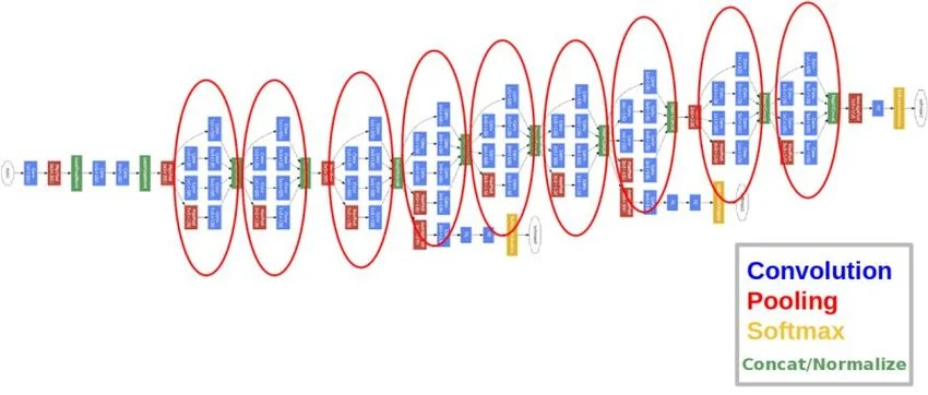
GoogleNet​

• Accurary: top-5 test erorr rate of 6.7%
• Close to human level performance
• 22 layer deep CNN
• Optimizer: RMSProp
• Total Trainable Parameters: ~4 million (Significantly reduced)
• A novel inception module was introduced

Inecption Module​

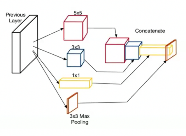
• Use filters with different size together
• Use different types of layers (CONV, POOL etc.) together
• It leads to better performance and efficiency but complicated architecture.

1X1 Convolution​

Input image ($6 \times 6 \times 1$), 1x1 kernel, and output can be declared as:

For channel reduction with a 1x1 convolution, each spatial location $(i,j)$ is a vector:

One 1x1 layer with 128 filters is a matrix:

At each location, output channels are computed by matrix multiplication:

So the shape changes as:

If we flatten all spatial positions ($64\times64=4096$):

Inception V2 and V3​

• V1 (GoogleNet): Replace one 5x5 conv with two stacked 3x3 conv layers.
  • Number of parameters: $5^2=25$ vs. $2\times3^2=18$ (about 28% reduction)
• V2: Factorize an $n\times n$ conv into $1\times n$ and $n\times1$ convs.
  • For $3\times3$: $3^2=9$ vs. $3+3=6$ (about 33% reduction)
• V3: Use more aggressive factorization and branch design (e.g., $1\times7$ and $7\times1$), plus efficient grid-size reduction.
  • Improves the accuracy-efficiency tradeoff while keeping computation manageable

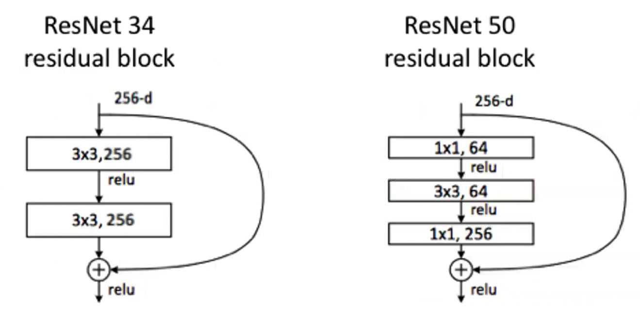
ResNet​

Deep Residual Networks, skip connections, and identity mappings

• Enabled the development of the much deeper networks
• ResNet is composed of residual blocks were introduced to address the vanishing gradient problem in deep networks.
  • Degradation problem: adding more layers eventually have negative effect on the final performance

High-Churn Files​

git log --format=format: --name-only --since="1 year ago" | sort | uniq -c | sort -nr | head -20

• Shows the most frequently changed files in the last year.
• These files often represent areas of the codebase with the highest maintenance burden.
• The top files can be cross-analyzed with bug hotspots to identify the highest-risk parts of the system.

Code Ownership and Bus Factor​

git shortlog -sn --no-merges

• Shows the number of commits by each author, excluding merge commits.
• If one person accounts for more than 60% of commits, the project may have a bus factor risk.
• If a top contributor has not been active in the last 6 months, it may indicate a maintenance gap.
• With only 3 out of 30 contributors active over the past year, this suggests a knowledge discontinuity caused by developer turnover.
• However, if the team uses squash merges, the commit history may be misleading for this analysis.

Bug Hotspots​

git log -i -E --grep="fix|bug|broken" --name-only --format='' | sort | uniq -c | sort -nr | head -20

• Shows the top 20 files with the most bug-related commits.
• By comparing this list with the high-churn files, we can identify code that is both frequently changed and bug-prone.
• While the accuracy depends on the quality of commit messages, even an approximate bug hotspot map can still be useful.

Development Velocity: Acceleration or Stagnation​

git log --format='%ad' --date=format:'%Y-%m' | sort | uniq -c

• Monthly commit counts provide a visual view of project activity over time.
• A consistent or increasing commit frequency suggests healthy development.
• A sudden drop, such as a 50% decrease in commits within a month, may signal the departure of key contributors or a shift in project focus.
• A sustained decline over 6-12 months suggests a loss of team momentum, while periodic spikes followed by stagnation may indicate a batch-style release pattern.
• In one real-world case, a CTO recognized from a commit velocity chart that a specific point in time aligned with the departure of a senior engineer.
• This data reflects not just code activity, but team dynamics.

Reverts, Hotfixes, and Firefighting Signals​

git log --oneline --since="1 year ago" | grep -iE 'revert|hotfix|emergency|rollback'

• Measures the frequency of urgent fixes and recovery actions.
• A few incidents per year are normal, but incidents every two weeks may signal a lack of trust in the deployment process.
• This often indicates deeper issues such as unstable tests, the absence of a staging environment, or complex rollback procedures.
• A result of zero may indicate either a stable codebase or poorly labeled commit messages.
• Crisis patterns tend to be clearly visible, and their mere presence is often enough to assess operational reliability.

Boolean Functions​

$f: \{0,1\}^n \to \{0,1\}$

• $n=1$
• Constant: smae output for all inputs ($f_0$ and $f_3$).
• Balanced: outputs 0 for exactly half, 1 for the other half ($f_1$ and $f_2$).
• In the worst case, need $2^{n-1}+1$ quries to decide which type $f$ is exponetial in $n$.

The Quantum Oracle​

• Traditional Oracle: black box that computes $f$.
• Query complexity: number of queries to the oracle needed to solve a problem.

$x \xrightarrow{O_f} f(x)$

• Quantum Oracle: unitary operation that encodes $f$.

$U_f \ket{x}\ket{y} = \ket{x}\ket{y \oplus f(x)}$

• First register: input $x$.
• Second register: auxiliary qubit initialized to $\ket{0}$ or $\ket{1}$.
• Oracle don't change $x$, but flips $y$ if $f(x)=1$.
  • $0 \oplus 0 = 0$
  • $0 \oplus 1 = 1$
  • $1 \oplus 0 = 1$
  • $1 \oplus 1 = 0$
• $f(x) = 0$: $y$ unchanged.
• $f(x) = 1$: $y$ flipped.
• Example:
  • $\ket{x}\ket{0}$
  • $U_f \ket{x}\ket{0} = \ket{x}\ket{0} \oplus \ket{f(x)} = \ket{x}\ket{f(x)}$.
  • if $f(x) = 0$: $\ket{x}\ket{0}$.
  • if $f(x) = 1$: $\ket{x}\ket{1}$
• so that it ignores the input $x$ and only flips the second qubit if $f(x)=1$.
• it can be reversed: $(y \oplus f(x)) \oplus f(x) = y$.

Phase Kickback​

• Prepare the scratch qubit in $\ket{-} = \frac{1}{\sqrt{2}}(\ket{0} - \ket{1})$.
  • $U_f \ket{x}\ket{-} = \frac{1}{\sqrt{2}}(U_f \ket{x} \ket{0} - U_f \ket{x} \ket{1})$
  • $= \frac{1}{\sqrt{2}}(\ket{x} \ket{0 \oplus f(x)} - \ket{x}\ket{1 \oplus f(x)})$
  • if $f(x) = 0 \rightarrow \\ \frac{1}{\sqrt{2}}(\ket{x}\ket{0 \oplus 0} - \ket{x}\ket{1 \oplus 0}) \\ = \frac{1}{\sqrt{2}}(\ket{x}\ket{0} - \ket{x}\ket{1}) \\ = \ket{x} \frac{1}{\sqrt{2}}(\ket{0} - \ket{1}) \\ = \ket{x}\ket{-}$.
  • if $f(x) = 1 \rightarrow \\ \frac{1}{\sqrt{2}}(\ket{x}\ket{0 \oplus 1} - \ket{x}\ket{1 \oplus 1}) \\ = \frac{1}{\sqrt{2}}(\ket{x}\ket{1} - \ket{x}\ket{0}) \\ = - \ket{x} \frac{1}{\sqrt{2}}(\ket{0} - \ket{1}) \\ = -\ket{x}\ket{-}$.
    • it doesn't matter where the phase is, it can be moved around:
    • $\alpha(\ket{\psi} \otimes \ket{\phi}) = \alpha\ket{\psi} \otimes \ket{\phi} = \ket{\psi} \otimes \alpha\ket{\phi}$.
• if we put the second register to $\ket{-}$, $f(x)$ will be encoded in the phase of the first register.

$\ket{x}\ket{-}\mapsto (-1)^{f(x)} \ket{x} \ket{-}$

• The function's output has been "kicked back" into the phase of the first register, while the second register remains unchanged.

The Deutsch Problem​

• Given a boolean function $f:\{0,1\}^{n} \to \{0,1\}$, determine if $f$ is constant or balanced.
• Constant: same output for all inputs.
• Balanced: outpus 0 for half the inputs and 1 for the other half.

1. Prepare $\ket{0}\ket{1}$.
2. Apply $H$ to both qubits $\to \ket{+}\ket{-}$.
3. Apply oracle $U_f$.
4. Phase kickback encodes $f$ in the input phase.
5. Apply $H$ to input qubit, then measure.

• One query to the oracle is sufficient to determine if $f$ is constant or balanced.
• if measure 0: $f$ is constant.
• if measure 1: $f$ is balanced.

Deustch-Jozsa Algorithm​

The direct generalization for any $n$-bit boolean function.

1. Input register $n$ qubits: Initialize qubits in $\ket{0}$ and apply $H$ gate to each one.
2. Scratch Qubit $1$ qubit: Initialize in $\ket{1}$ with $X$ and then apply an $H$ gate.
3. Oracle: Apply $U_f$ to the input and scratch registers (All qubits).
4. Final Hadamards: Apply $H$ to input qubits.
5. Measurement: Measure the input register.

• if all qubits returned $0$: $f$ is constant.
• if any qubit returned $1$: $f$ is balanced.

How it works​

• The initial state is

$\ket{00 \cdots 0} \ket{1}$

• After applying $H$ gates to the input and scratch registers, we get

$\ket{00 \cdots 0} \rightarrow \frac{1}{\sqrt{2^n}} \left( \ket{00 \cdots 0} + \ket{00 \cdots 1} + \cdots + \ket{11 \cdots 1} \right)$

• The input register is in a superposition of a computational states containing all possible inputs to $n$-bit string.
• The last qubit hasn't changed from $n = 1$ case, so it is in the state $\ket{-}$.
  • $H\ket{1} = \ket{-}$
• The definition of the oracle was generic for any bit string: $U_f \ket{x}\ket{-} = (-1)^{f(x)} \ket{x} \ket{-}$
• The phase-kickback puts a phase in front of each term in the input register that depends on the output of the function $f$: $\frac{1}{\sqrt{2^n}}\big(\;(-1)^{f(00\ldots0)}|00\ldots 0\rangle+ \cdots +(-1)^{f(11\ldots1)}|11\ldots 1\rangle\;\big)$
  • The scratch qubit remains in $\ket{-}$, so we can ignore it for the rest of the algorithm.
• Constant case
  • if $f$ is constant, then all the phases are the same, either $+1$ or $-1$:
  • $f(00 \cdots 0) = f(00 \cdots 1) = \cdots = f(11 \cdots 1) = 0$
  • $f(00 \cdots 0) = f(00 \cdots 1) = \cdots = f(11 \cdots 1) = 1$
  • The phse in front of every computational state is the same, Either $+1$ or $-1$.
  • Before the second application of the $H$ gates, the state of the input register is:
  • $\pm \frac{1}{\sqrt{2^n}} \left( \ket{00 \cdots 0} + \ket{00 \cdots 1} + \cdots + \ket{11 \cdots 1} \right)$
  • In measurement, in either case, the probability to obtain $P(00 \cdots 0) = 1$
  • A constant function deterministically returns all zeros with a single query.
• Balanced case
  • we are promised the function is either constant or balanced, so there are equal number of $+1$ and $-1$ phases. so we don't need to consider this case.
  • If the measurement produces anything but all zeros, we know with certainty the function is not constant, so it must be balanced.
  • There are a lot of balanced function, but half the terms in the superposition will exactly have a $-1$ phase.
  • It's clearly orthogonal to the state with all ones in superposition.
  • Appllying $H$'s will change the state to some other superpostiion, or perhaps a unique computational state.
  • But, orthogonality to $\ket{00 \cdots 0}$ must remain.
  • A balenced function deterministically returns a state with at least one entry as $1$, with a single query.

One quantum query vs $2^{n-1} + 1$ classical queries. It is an algorithm that puts all inputs into superposition at once, encodes the function values as phases, and then uses interference to distinguish between constant and balanced functions.

Buildling Oracles​

Multi-Controlled and Anti-Controlled Gates​

• build $U_f$ that applies $X$ to the output qubit exactly when $f(x) = 1$.
  • if $n=2$, the multi-controlled $X$ gate is a Toffoli gate.
  • $x=11$ is the only input that gives $f(x) = 1$, so we can use a Toffoli gate with controls on the first two qubits and target on the output qubit.
    • This is because the Toffoli gate will flip the output qubit if and only if both control qubits are $\ket{1}$, which corresponds to the input $x=11$.
  • if $x=00$ is the only input that gives $f(x) = 1$, we can use an anti-controlled Toffoli gate, which applies $X$ to the target qubit if both control qubits are $\ket{0}$.
    • This is because the anti-controlled Toffoli gate will flip the output qubit if and only if both control qubits are $\ket{0}$, which corresponds to the input $x=00$.
    • Applying $X$ gates to the two control qubits, then applying a Toffoli gate, and then applying $X$ gates again to the control qubits will effectively create an anti-controlled Toffoli gate.

• A multi-controlled $X$ gates ($C^nX$) flips the target only all control qubits are $\ket{1}$.
• To target a specific input $x$:
  • Place $X$ gates on each qubit $i$ where $x_i = 0$. (anti-control)
  • Apply $C^nX$.
  • Undo the $X$ gates.
• For $n$ qubits, it can be generalized to perform an $X$ gate (or any $U$) with $n$ control qubits, requireing $n-1$ extra scratch qubits and $2(n-1)$ Toffoli gates.
• Whenever scratch qubits are invoked, always see a symmetric pattern of gates.
• $U_{f8} U_{f1} \ket{x}\ket{y} = \ket{x}\ket{y \oplus f_1(x) \oplus f_8(x)} = \ket{x}\ket{y \oplus f_9(x)}$

1. The computation is done using the scratch qubits.
2. The answer is copied to the target or output register
3. The computation is inverted to reset the scratch qubits to $\ket{0}$.

• called "uncomputation", ensures the scratch qubits are returned to their initial state.
• no input or output qubits are entangled with the scratch qubits at the end of the algorithm.

Implementing Deutsch-Jozsa​

def random_oracle(n):
    # Circuit object to hold the gates
    circuit = qiskit.QuantumCircuit(n + 1)

    # With 50% probability, return a constant oracle
    if np.random.randint(0, 2):
        qasm = ""
        # another 50:50 chance of it being a 1 instead of 0 oracle
        if np.random.randint(0, 2):
            qasm += f"x q[{n-1}];"
        return qasm, "constant"

    # A balanced function has half the inputs as 0
    # Randomly select where those are
    zero_strings = np.random.choice(range(2**n),int(2**(n-1)),replace=False)

    for string in zero_strings:

        # Convert base 10 to 2
        bitstring= f"{string:0b}"

        # X gates for 0 locations
        for xi, bit in enumerate(reversed(bitstring)): # enumerate iterates through the list as well as the index in the list
            if bit == "1":
                circuit.x(xi)

        # C^n X gate
        circuit.mcx(list(range(n)), n)

        # X gates for 0 locations
        for xi, bit in enumerate(reversed(bitstring)):
            if bit == "1":
                circuit.x(xi)

    transpiled_circuit = qiskit.transpile(circuit, basis_gates=["u1", "u3", "u2", "cx"])
    qasm = qiskit.qasm2.dumps(transpiled_circuit)[47:]
    return qasm, "balanced"

OPENQASM 2.0;
qreg q[3];
creg c[2];

x q[2];
h q[0];
h q[1];
h q[2];

/* oracle for f(00)=1 */
x q[0];
x q[1];
ccx q[0],q[1],q[2];
x q[0];
x q[1];

/* oracle for f(11)=1 */
ccx q[0],q[1],q[2];

h q[0];
h q[1];

measure q[0] -> c[0];
measure q[1] -> c[1];

OPENQASM 2.0;
qreg q[n+1];
creg c[n];

x q[n];
h q[0];
h q[1];
...
h q[n];
/* oracle U_f */
h q[0];
h q[1];
...
h q[n-1];
measure q[0] -> c[0];
...
measure q[n-1] -> c[n-1];

Bernstein-Vazirani Algorithm​

• Given $f_s: \{0,1\}^n \to \{0,1\}$ defined as $f_s(x) = s \cdot x \mod 2$
  • where $s$ is an unknown $n$-bit string and $x$ is the input.
• The goal is to determine the hidden string $s$ as few queries as possible.
• Classically: query $f$ with input $e_0 = 00 \cdots 01$, $e_1 = 00 \cdots 10$, ..., $e_{n-1} = 10 \cdots 00$ to get each bit of $s$.
  • Total $n$ queries.
• Quantum: use the exact same circuit as Deutsch-Jozsa.
  • $U_{f_s} \ket{x} = (-1)^{s \cdot x} \ket{x}$.
    • where we can ignore the output register in the $\ket{-}$ state.
    • For $n =1$, the state after the oracle before the final $H$ gate is:
      • $\frac{1}{\sqrt{2}} \left( \ket{0} + (-1)^{s} \ket{1} \right)$
    • which is $\ket{+}$ if $s=0$ and $\ket{-}$ if $s=1$.
  • Applying $H$ to this state returns $s$:
    • $H \frac{1}{\sqrt{2}} \left( \ket{0} + (-1)^{s} \ket{1} \right) = \ket{s}$.
  • The measurement deterministically reveals $s$.

n=2 case​

• $s = s_1s_0$ and $x = x_1 x_0$
• $\rightarrow s\cdot x = s_1x_1 + s_0 x_0$

this factorized into:

$\frac{1}{\sqrt{2}}\big(\ket 0 + (-1)^{s_1}\ket 1\big)\otimes \frac{1}{\sqrt{2}}\big(\ket 0 + (-1)^{s_0}\ket 1\big).$

this reduces the same agument as $n=1$ for each qubit where after the final $H$ gates, the state becomes:

Implemnting Bernstein-Vazirani​

• $\mathbb{I}$ if $s = 0$ and $CNOT$ if $s = 1$.
• To implement $f_{s}(x) = s \cdot x$, we can use a CNOT from qubit $i$ to the scratch qubit if $s_i = 1$.

import numpy as np
from qiskit import QuantumCircuit, transpile
from qiskit_aer import AerSimulator


def bv_query(n, secret=None):
    # Build oracle for f_s(x) = s · x
    # q[0]..q[n-1] = input register
    # q[n] = scratch/output qubit

    if secret is None:
        value = np.random.randint(0, 2 ** n)
        secret = format(value, f"0{n}b")
    else:
        secret = secret.zfill(n)

    oracle = QuantumCircuit(n + 1, name="Uf")
    for index, bit in enumerate(reversed(secret)):
        if bit == "1":
            oracle.cx(index, n)

    return oracle, secret


def bernstein_vazirani_circuit(n, secret=None):
    # Build full Bernstein-Vazirani circuit
    oracle, secret = bv_query(n, secret)

    qc = QuantumCircuit(n + 1, n)

    # Prepare scratch qubit in |->
    qc.x(n)

    # Apply Hadamards to all qubits
    for i in range(n + 1):
        qc.h(i)

    # Apply oracle
    qc.compose(oracle, inplace=True)

    # Apply final Hadamards to input register
    for i in range(n):
        qc.h(i)

    # Measure input register
    for i in range(n):
        qc.measure(i, i)

    return qc, secret


def run_bernstein_vazirani(n, secret=None, shots=1):
    qc, secret = bernstein_vazirani_circuit(n, secret)

    simulator = AerSimulator()
    compiled = transpile(qc, simulator)
    result = simulator.run(compiled, shots=shots).result()
    counts = result.get_counts()

    measured = max(counts, key=counts.get)
    recovered = measured[::-1]

    return qc, secret, recovered, counts


# Example
qc, secret, recovered, counts = run_bernstein_vazirani(5, "01101")
print(qc.draw())
print("Secret   :", secret)
print("Measured :", recovered)
print("Counts   :", counts)

OPENQASM 2.0;
qreg q[6];
creg c[5];

x q[5];
h q[0];
h q[1];
h q[2];
h q[3];
h q[4];
h q[5];

cx q[0],q[5];
cx q[2],q[5];
cx q[3],q[5];

h q[0];
h q[1];
h q[2];
h q[3];
h q[4];

measure q[0] -> c[0];
measure q[1] -> c[1];
measure q[2] -> c[2];
measure q[3] -> c[3];
measure q[4] -> c[4];

Summary​

• There are $2^{2^n}$ possible Boolean functions from $\{0,1\}^n$ to $\{0,1\}$.
• A Boolean function is balanced if it outputs 1 on exactly half of the inputs, that is, on $2^{n-1}$ out of the $2^n$ possible inputs.
• In Deutsch’s algorithm with $n=1$, only 1 quantum query is needed to distinguish a constant function from a balanced function.
• A quantum oracle for $f$ is defined as the unitary $U_f:\ |x\rangle|y\rangle \mapsto |x\rangle|y\oplus f(x)\rangle.$
• Every XOR-based function of the form $f(x)=x_j\oplus x_k\oplus\cdots$ that depends on at least one input bit is balanced.
• Using multi-controlled $X$ gates, together with anti-controls when needed, we can implement an oracle for any Boolean function.
• The phase kickback multiplies the state by the phase factor $(-1)^{f(x)}$, so the phase changes exactly when $f(x)=1$.
• If these questions were stored in a Python list called questions, then the 8th question would be questions[7].
• Applying Hadamard gates to $n$ qubits initialized in $|0\rangle$ produces an equal superposition over all $2^n$ computational basis states.
• In Deutsch–Jozsa for $n>1$, measuring all input qubits as 0 means that $f$ is constant.
• Bernstein–Vazirani solves the hidden-string problem $f(x)=s\cdot x$ with 1 quantum query.
• A multi-controlled $X$ gate with 3 controls can be implemented using scratch qubits and 4 Toffoli gates.
• Applying $U_{f_1}$ followed by $U_{f_2}$ yields an oracle whose action on the scratch qubit corresponds to $f_1(x)\oplus f_2(x)$.
• Uncomputation resets scratch qubits to their initial states by applying the inverse of the computation, which means reversing the order of the steps.
• Multi-controlled gates with more than one control can be decomposed into simpler gates, but in general this requires more than just $CX$ and $X$; single-qubit gates are also needed.

Data Preparation​

• Small Dataset (Range: 100 to 100,000 samples)
  • Train/Valid/Test: 60/20/20
  • Train/Test: 70/30
• Large Dataset (Range: 500,000 to 1M+ samples)
  • Train/Valid/Test: 98%/10,000/10,000
  • usaully more traning data is get better performance.
• Rule of Thumb: Validation and Test set should com from the same distribution.

Bias and Variance​

• Bias: A value that allows to shift the activation function to left or right to better fit the data.
  • With bias the curve/line will not always pass through origin
  • can get a better fit to training data
• Variance: The sensitivity of the model to small fluctuations in the training data.
  • The change in prediction accuracy of ML model between training data and test data.
  • Model with high variance pays a lot of attention to tranining data and does not generalize on the data which is has not seen before.
  • With high variance, model perform very well on training data but poorly on test data.

• High Bias
  • High training error, underfitting
  • Validation/test error nearly same as train error
  • Potential things to try:
    • Increase features
    • Make ML model more complicated
    • Decrease Regularation parameters
• High Variance
  • Low tranining error, overfitting
  • High validation/test error
  • Potential things to try:
    • Increase dataset size
    • Reduce input features
    • Increasing Regularization parameter

Accuracy​

• Bayesian Optimal Error (BOE): Best optimal error that can be achieved by any model on a given dataset.
• Human-Level performance:
  • Humans are very good at a lot of tasks
  • Can get labelled data from humans to help improve the model performance
  • Gain insights from manual error analysis

Regularization​

• a technique which makes slight modifications to the learning algorithm such that the model generalizes better on the unseen data.
• Update the loss/cost function by adding a regularization term
  • $\text{Loss function} = \text{Loss} + \text{Regularization term}(\lambda)$
  • Due to $\lambda$, the weight matrices will decrease, assuming a neural network with smaller weight matrices leads to simpler model.
  • Regularization penalizes the weights matrices of the nodes
• L2 regularization
• L1 regularization
• Dropout

L2 Regularization​

$\text{Cost function} = \text{Loss} + \frac{\lambda}{2m} \sum_{j=1}^{n_x} w_j^2$

• $\lambda$ is a hyper-parameter
• as weight decay, as it forces the weight to decay towards zero, but not exactly zero.

L1 Regularization​

$\text{Cost function} = \text{Loss} + \frac{\lambda}{2m} \sum_{j=1}^{n_x} |w_j|$

• Penalize the absolute value of the $w$
• Weight may reduce to zero
• Useful in compressing a model (sparse model)

Dropout​

• It produces good reuslts and most popular regularization technique in deep learning.
• At every iteration, it randomly selects and drops some nodes and remove all the connections to those nodes.
• Each iteration has a different set of nodes.

Data Augmentation​

• Simple way to reduce overfitting is to increase size of tranining dataset.
• By creating more sample using the existing set and applying the following simple operations
  • Flip
  • Rotate
  • Scale
  • Crop
  • Translate
  • Gaussian Noise

Cutout​

• Simple regularization technique of randomly masking out square regions of input during training.
• Patch size: 16x16 to 64x64
• Fill value: 0 or mean pixel value
• Patches: 1-3 per image

Mixup​

• Trains a neural network on convex combinations of pairs of examples and their labels.
• It regularizes the neural network to favor simple lienar behavior in-between training examples.
• Image A ($\lambda = 0.55$) + Image B ($\lambda = 0.45$) = Blended Output

CutMix​

• Patches are cut and pasted among training images, where the ground truth labels are also mixed proportionally to the area of the patches.
• Image A + Image B (Patch) = Pasted Patch Output.

Random Agumentation​

• A set of augmentation operations is defined, and a random subset of these operations is applied to each image during training.
• Identity, AutoContrast, Equalize, Rotate, Solarize, Color, Posterize, Contrast, Brightness, Sharpness, ShearX/Y, TranslateX/Y

Generative Adversarial Networks (GANs)​

• Able to generate images which look similar to the original ones
• Proven to be very effective in data augmentation, especially when the dataset is small.

Neural Style Transfer​

• Using CNN to separate style
• Transfer style to different image

주제 선정​

• 박사과정 4년 중 1.5년은 읽기만 해야한다.
• Area of Interest (AOI)는 내가 좋아하는 걸 해야 버틸 수 있다.
• 그리고 그 1.5년 뒤에는 Research Question이 나올 것이다.
• 4년 내의 논문에서 Future Work를 취합하자.

좋은 연구 주제​

• Government
  • Originality of content, document
  • How can differntiate from generated content?

Master leading to PhD​

• UTS: feature research students

논문​

• Abstract가 흥미있으면 Conclusion을 읽고, 그 다음 관련 내용이면 전체를 읽어야한다.
• 공식을 처음부터 이해하려고 하지 말자.
• 2022년 이후 (4개년까지만) 논문을 읽어야한다.
  • 왜냐면 박사과정이 4-5년이니까.

Computer Vision​

• Classification
• Classification with Localization
• Object Detection

Convolutional Neural Networks (CNN)​

1. Convolutional Layer (CONV)
2. Pooling Layer (POOL)
3. Fully Connected Layer (FC)

Convulutional Layer (CONV)​

• The first layer to extraact features from an input image
• Core buildling block of a CNN
• Convolutions are basic operation in this layer
• A number of filters (e.g. edge detectors) are applied to the input image.

Padding​

• Padding is used to control the spatial size of the output feature maps.
• Negative values at the edges can naturally arise because of padding, and they usually are not a big problem because activation functions and later layers come afterward.
• Input Matrix dimension: $n \times n \times c$ (height, width, channels)
• Filter size: $f \times f$
• Padding ($P$): 1, number of pixels added to the border of the input
• $(n \times n) * (f \times f) \to (n + 2P - f + 1) \times (n + 2P - f + 1)$
  • Example: $5 \times 5$ input with $3 \times 3$ filter and padding of 1 results in a $5 \times 5$ output feature map.
• if input and output matrix dimensions are the same, then $P = \frac{f - 1}{2}$.
• Valid padding ($P = 0$): No Padding
• Same padding ($P = \frac{f - 1}{2}$): Output size and input size is same, this requires appropriate padding.

Stride​

• It is the number of pixels by which slide the filter across the input image.

No Padding Strides	Stride with Padding

• Github: vdumoulin/conv_arithmetic
• Input Matrix dimension: $n \times n$
• Filter size: $f \times f$
• Padding: $P$
• Stride: $S$
• Output Size = $\left\lfloor \frac{n + 2P - f}{S} + 1 \right\rfloor \times \left\lfloor \frac{n + 2P - f}{S} + 1 \right\rfloor$
  • Example: Input Matrix dimension: $5 \times 5$, Filter size: $3 \times 3$, Padding: $1$, Stride: $2$ results in an output size of $2 \times 2$.

Pooling Layer (POOL)​

• Down sampling operation which reduces the dimensionality of a matrix.
• Reduces the number of parameters for large image, but retain the valuable information.
• Max pooling
• Average pooling
• Sum pooling

Fully Connected Layer (FC)​

• a traditional Multi-layer Perception (MLP) layer
• For multi-class classification, usually Softmax activation is used.
• Softmax ensures the output.
• Output of the CONV and POOL layers represent a high level features of the Input image.
• The FC layer takes these features to classify the input image into the desired output classes.

Logistic Regression as Neural Network​

• if $y = 1$
  • $L = -\log(\hat{y})$
  • if $\hat{y} \to 1$, then $L \to 0$ (low loss)
  • if $\hat{y} \to 0$, then $L \to \infty$ (high loss)
• if $y = 0$
  • $L = -\log(1 - \hat{y})$
  • if $\hat{y} \to 0$, then $L \to 0$ (low loss)
  • if $\hat{y} \to 1$, then $L \to \infty$ (high loss)

Gradient Descent​

• it is an iterative approach for error correction in a machene learning model
• Find $w$ and $b$ that will minimize $GD(w, b)$ (requires Loss/Cost function)

1. Initialize $w$ and $b$
2. Perform Forward pass operation/calculations
3. Compute Loss/Cost function $L(a, y)$
4. Compute change in $w$ and $b$ (Take the partial derivative of the cost function with respect to Weights and bias $dw$ and $db$)
5. Update $w$ and $b$ ($w := w - \alpha dw$ and $b := b - \alpha db$)
6. Repeat from Step 2 with new values of $w$ and $b$ for 'n' number of iterations.

• $\alpha$ is the learning rate (hyperparameter) that controls how much we are adjusting the weights and bias of our model with respect to the loss gradient. It is a small positive value (e.g., 0.01, 0.001) that determines the step size at each iteration while moving toward a minimum of the loss function.

Gradient Descent Types​

• Batch Gradient Descent (BGD)
• Stochastic Gradient Descent (SGD)
• Mini-batch Gradient Descent (MBGD)

Batch Gradient Descent (BGD)​

1. Process each input sample and find the cost
2. Find the average cost oveer all input samples
3. Update $w$ and $b$ and repeat the steps for "n" epochs(iterations)

• Disadvantages:
  • It uses the complete dataset to calculate the gradients at every steps
  • Slow when training data is large
  • Difficult to find the learning rate
  • Difficult to ascertain the number of epochs(iterations)

Stochastic Gradient Descent (SGD)​

Due to the random nature, the algorithm is much less regular than BGD.

1. Process a random input sample and find the cost.
2. Update $w$ and $b$, and repeat the steps for "n" iterations on the training samples.

• Advantages:
  • Computes gradient based on single input sample, which is memory efficient.
  • Much faster compared to BGD.
  • Possible to train on large datasets.
  • Randomness is helpful to escape local minima.
• Disadvantages:
  • Might not reach the optimal value, but very close to it.
    • Simulated annealing: Reduce the learning rate gradually
    • Create a Learning Schedule to determine the learning rate at each iteration.

Mini-batch Gradient Descent (MBGD)​

1. Divide the tranining set into mini-batches of size $n$ (e.g., 64, 128, 256).
2. Process all the samples in a mini-batch and find the average cost
3. Update $w$ and $b$, and repeat the steps for "n" iterations/epoches on the traning samples.

• Advantages:
  • Computes gradient based on small sets of input smaple
  • Much faster compared to BGD.
  • Possible to train on large dataset.
  • Performance boost on matrix operations using GPUs.
  • Might not reach the optional value but, very close to it and possibly better than SGD.
• Disadvantages:
  • It may be harder to escape the local minima compared to SGD.

Exponentially Weighted Averages​

• One of the popular algorithm for smoothing sequential data (time series data), aka. moving average.
• Weight the number of observations and using their average

$V_t$ is approximate average over $\approx \frac{1}{1 - \beta}$ time steps.

• For $\beta = 0.9$, $V_t$ is average over the last 10 time steps.
• For $\beta = 0.98$, $V_t$ is average over the last 50 time steps.
• For $\beta = 0.5$, $V_t$ is average over the last 2 time steps.

Optimizers​

SGD with Moementum​

At iteration $t$:

• Calculate $dw$ and $db$ on the current mini-batch (Hyper parameters: $\alpha$ and $\beta$)
• Update the velocity:
  • $V_{dw} = \beta V_{dw} + (1 - \beta) dw \rightarrow V_t = \beta V_{t-1} + (1 - \beta) \theta_t$
  • $V_{db} = \beta V_{db} + (1 - \beta) db$
• Update parameters:
  • $w := w - \alpha V_{dw}$
  • $b := b - \alpha V_{db}$

RMSProp​

• Root Mean Square Propagation.
• Unpublished adaptive learning method by Geoffrey Hinton.
• Reduces oscillation but in a different way than Momentum.
• Divides the learning rate by an exponentially decaying average of squared gradients.
• Calculate $dw$ and $db$ on the current mini-batch
  • $S_{dw} = \beta S_{dw} + (1 - \beta) dw^2$
  • $S_{db} = \beta S_{db} + (1 - \beta) db^2$
• Update parameters:
  • $w := w - \alpha \frac{dw}{\sqrt{S_{dw}} + \epsilon}$
  • $b := b - \alpha \frac{db}{\sqrt{S_{db}} + \epsilon}$
  • $\epsilon$ is a small number to prevent division by zero (e.g., $10^{-8} \text{ to } 10^{-10}$)

Adam​

• Adaptive Moment Estimation
• Combination of RMSProp and Momentum
• Work well for a wide range of non-convex optimization problems in machine learning.
• Calculate $dw$ and $db$ on the current mini-batch
  • $V_{dw} = \beta_1 V_{dw} + (1 - \beta_1) dw \leftarrow Momentum, \beta_1$
  • $V_{db} = \beta_1 V_{db} + (1 - \beta_1) db$
  • $S_{dw} = \beta_2 S_{dw} + (1 - \beta_2) dw^2 \leftarrow RMSProp, \beta_2$
  • $S_{db} = \beta_2 S_{db} + (1 - \beta_2) db^2$
• Update parameters:
  • $w := w - \alpha \frac{V_{dw}}{\sqrt{S_{dw}} + \epsilon}$
  • $b := b - \alpha \frac{V_{db}}{\sqrt{S_{db}} + \epsilon}$
  • $\epsilon$ is a small number to prevent division by zero (e.g., $10^{-8} \text{ to } 10^{-10}$)
• Hyper parameter guide:
  • $\alpha = 0.001$
  • $\beta_1 = 0.9$: Momentum term
  • $\beta_2 = 0.999$: Moving weighted average
  • $\epsilon = 10^{-8}$: To prevent division by zero
• ensmallen.org

Learning Rate Decay​

• Speed-up the learning algorighm by slowing decreasing the learning rate $\alpha$ as the number of epochs increases.

Activation Functions​

• Getting the output of a layer in a neural network and applying a non-linear function to it.
  • Sigmoid: $\sigma(x) = \frac{1}{1 + e^{-x}}$
  • Tanh: $\tanh(x) = \frac{2}{1 + e^{-2x}} - 1$
  • Used for binary classification in the output layer.
• ReLU: $A(x) = \max(0, x)$
  • Rectified Linear Unit
  • Avoids and rectifies vanishing gradient problem
  • Best used in hidden layers
  • Computationally less expensive than sigmoid and tanh
• Softmax: $S(x_i) = \frac{e^{x_i}}{\sum_{j} e^{x_j}}$
  • Turns numbers in probabilities that sum to 1.
  • Used for multi-class classification in the output layer.