FSD +007

· 3 min read

Collection

a data sturcucture that groups multiple elemtns togehter logically.

  • referenced by the collection name, and its elements are accessed using indexing or look up methods.
  • some collections allow dynamic sizing, expanding and shrinking with the data, others have a fixed size.
  • can store mixed data types.
    • Java collections are typically type-safe using generics.
    • Python uses dynamic typing.

Python List

mylist = ["Tom", 30, 112.5]
len(mylist)
mylist[index]
mylist.append(item)
mylist.insert(index, item)
# returns a slice of a list from first to last-1
mylist[first:last]
mylist.index(item)

# replaces items from first to last-1 with a list
mylist[first:last] = [list-values]
# adds list 2 at the end of list 1
mylist = list1 + list2
# adds list 2 at the end of list 1
list1.extend(list2)

mylist.remove(item)
mylist.pop(index)
mylist.pop()
del mylist[index]
del mylist
mylist.clear()

# Sorts the list alphanumerically, ascending
mylist.sort()
mylist.sort(reverse =True)
mylist.reverse()
mylist.count()

Python Set

  • unordered, not indexed.
  • mutable, unique.
myset = { 'hello', 5, True, 3.5 }

for x in myset:
print(x)

myset.add(item)
# Merges myset iwth the otherset, rtaining unique values
myset.update(otherset)
# Adds other set items to a set (only unique items are retained)
mynewset = myset.union(otherset)
# Retain only the items that exists into set1 and set2
myset = set1.intersection(set2)

# report error if item not found
myset.remove(item)
myset.discard(item)

myset.pop()
myset.clear()
del myset

Python Tuple

  • a cllection of items of any type
  • ordered, indexed
  • unchangable, once a tuple is created the elemets are fixed
mytuple = ("Tom", 30, 112.5)
len(mytuple)
mytuple[index]
mytuple[first:last]
mytuple = tuple + tuple2

Python Dictionary

  • a collection of items represented as key-value pairs
  • unordered, indexed by uniaue keys
  • itmes are mutable
  • allow duplicate values but not duplicate keys
mydata = {
"name": "Tom",
"age": 30,
"role": "admin"
}

mydata.keys()
len(mydata)
mydata[key]
mydata[key] = new-value
del mydata[key]
del mydata

# Deletes an entry associated with key
val = mydata.pop(key)
# Updates/Inserts { k: v } entry into the dictionary
mydata.update({ k: v })

Java List

  • an interface of the Java Collection Framework (JCF)
  • cannot be instantiated.
  • common implementation of List interface
    • ArrayList
    • LinkedList
List<Integer> numbers = new ArrayList<>();
List<String> names = new LinkedList<>();

numbers.get(0);
numbers.get(numbers.size() - 1);

names.get(indexOf("Hello"));
names.get(lastIndexOf("Hello"));

numbers.add(5);
names.remove("Hello");
names.remove(indexOf("Hello"));

numbers.removeAll(<another list>);
// set(2, 12) replaces the item at index 2 with 12
numbers.set(2, 12);

Java Set

  • an interface of the Java Collection Framework (JCF)
  • unordered, unique objects.
HashSet<String> names = new HashSet();
HashSet<String> names = new HashSet(Array.asList("Tom", "Jerry", "Mickey"));

HashSet<String> names = new HashSet();
ArrayList list1 = new ArrayList();
ArrayList list2 = new ArrayList();

list1.add("Tom");
list1.add("Jerry");

names.addAll(list1);
names.addAll(list2);

names.remove("Tom");
boolean isRemoved = names.remove("Tom");

for (String name : names) {
System.out.println(name);
}

Iterator<String> it = names.iterator();
while (it.hasNext()) {
System.out.println(it.next());
}

names.clear();
names.isEmpty();
names.contains("Tim");
names.size();
names.removeAll(set2);
names.containsAll(set2);
// Retain set2 elements and discard the rest
names.retainAll(set2);

Java Map

  • interface from java.util stores data as a keiy-value pairs
  • contain unique keys that are associated with specific values.
HashMap<Integer, String> people = new HashMap<>();
people.put(1, "Tom");
people.put(2, "Jerry");
people.put(3, "Mickey");

people.putIfAbsent(2, "Donald");
System.out.println(people.get(2));

people.put(2, "Lucy");
people.replace(2, "Amy");
people.remove(2);

System.out.prinln(people.keySet());
System.out.println(people.values());

people.clear();
people.isEmpty();
people.containsKey(2);
people.size();
people.getOrDefault(50, "Unknown");
// Checks if the value is mapped with one or more keys
people.containsValue("Jim");

Operation Patterns

  • Finding an item in a list: Using the lookup pattern
  • Finding multiple items in a list: Using the updated-lookup pattern
  • Removing certain items from a list: Using the remove-all pattern

Sentence structures

· 4 min read

Types of sentence structure

The secret to good writing is variation and using a mix of these types of sentences within your paragraphs in your written work.

  • Simple sentence
    • is one independent clause in a subject-verb pattern
    • e.g. The Australian government introduced an official carbon tax on 1 July 2012.
  • Compound sentence
    • is two independent clauses connected by a coordinating conjunction.
    • e.g. The Australian government introduced an official carbon tax on 1 July 2012, but this was met with opposition from the general public.
  • Complex sentence
    • consists of an independent clause and a dependent clause.
    • e.g. As the Australian government recognized the necessity to significantly reduce greenhouse gas emissions, it introduced an official carbon tax on 1 July 2012.
  • Compound-complex sentences
    • consists of more than one independent clause and one or more dependent clauses
    • e.g. As the Australian government recognized the necessity to significantly reduce greenhouse gas emissions, it introduced an offical carbon tax on 1 July 2012, but this was met with opposition from the general public.

Common sentence structure errors

Sentence fragments

  • A sentence fragment is missing some of its parts.
  • There are three main reasons why a sentence may be incomplete.
    • Missing subject
      • e.g Becoming extinct because of rising sea tempratures.
      • Correction: Phytoplankton could become extinct because of rising sea temperatures.
    • Missing verb
      • e.g. Significantly, one particular form of Western Australian finch.
      • Correction: Significantly, one particular form of Western Austrailan finch has decreased in numbers.
    • Incomplete thought
      • e.g. In a recent article about loss of habitat due to climate change.
      • Correction: In a recent article about loss of habitat due to climate change, Australian animals were shown to be particularly vulnerable.
  • Sentences beginning with words like so, as, because, who, which, that are often incomplete.

Run-on sentences

  • A run-on sentence occurs when two simple sentences are incorrectly joined. e.g. Poverty, famine and major public health problems around the developing world are important indicators of a changing climate these issues are not being addressed globally.
  • Use a joining or linking word such as and, but, or, nor, for, so, yet.
    • Correction: Poverty, famine and major public health problems around the developing world are important indicators of a changing climate, but these issues are not being addressed globally.
  • Make two separate sentences.
    • Correction: Poverty, famine and major public health problems around the devleoping world are important indicators of a chaing climate. These issues are not being addressed globally.

Lack of Meaning

  • Ensure that each sentence you write has clear meaning in English.
  • It must be fully understandable when read.
  • If you ware not sure if your sentence has clear meaning in English, perhaps think about rewriting it in a simpler and clearer way that you can fully understand (as will hopefully your reader).

Tips for writing

  • Consider the following example where each sentence follows a similar structure.
    • Topic Sentence: main point of the paragraph.
    • Supporting Sentence: Examples, evidence, or analysis.
    • Concluding Sentence: wrap up paragraph by linking to broader topic, or linking to the next paragraph or section.
  • This uniformity leads to a lack of cohesion, making the paragraph feel disjointed and somewhat monotonous.
    • e.g. Nursing education states that measures should be in place to avoid infection. Also, that infection rates tend to soar when hygiene standards decrease. Appropriate steps should be taken to decrease these risks. It is suggested that medical staff are educated to understand these risks.
    • Correction: Nursing educators argue that strict measures should be implemented to avoid infection in medical institutions. There is also much evidence to demonstrate that infection rates rise dramatically when hygiene standards begin to fall. Therefore, it is argued that appropriate steps need to be in place to decrease and minimize these potential risks. Furthermore, aggressive steps should be taken to ensure that all staff maintain effective hygiene and infection control.

Ref

VLA Test Review

· 6 min read

VLATest: Testing and Evaluating Vision-Language-Action Models for Robotic Manipulation

  • VLATest fuzzes 18,604 manipulation scenes (10 operators, 4 tasks) to systematically stress-test VLA robustness.
  • Seven VLA models show low success and brittleness to confounders, lighting/camera changes, unseen objects, and instruction mutations; larger pretraining helps.
  • Priorities: scale/augment demo data (incl. sim2real), use stepwise/CoT prompting & multi-agent setups, and expand benchmarks with online risk assessment.

Motivation & Gap

  • Problem: Current VLA models are typically evaluated on small, hand-crafted scenes, leaving general performance and robustness in diverse scenarios underexplored.
  • Goal: Introduce VLATest, a generation-based fuzzing framework that automatically creates robotic manipulation scenes to test performance and robustness of VLA models.

What Are VLA Models?

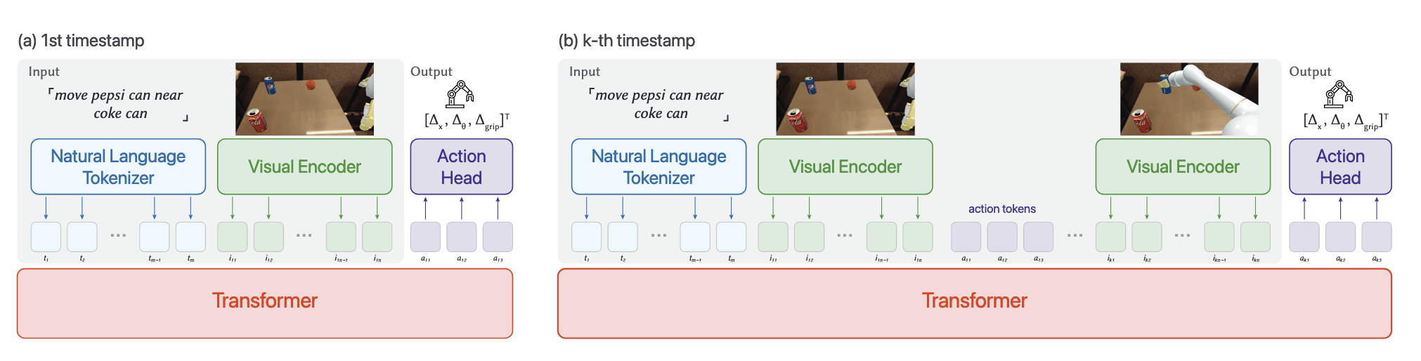
  • Vision-Language-Action (VLA) models take natural language instructions + camera images and output low-level robot actions (Δx, Δθ, Δgrip).
  • Inference loop: Tokenize text/image → transformer predicts action token A₁ → execute → append A₁ + new image tokens I₂ → predict A₂ → … until success or step limit.

VLA Architecture

Training & Evaluation

  • Training: (1) Train from scratch on robot demonstrations, or (2) fine-tune a large VLM (e.g., Llava) with >1B params pretraining.
  • Evaluation: Task-specific metrics (e.g., grasp, lift, hold for “pick up”), either in sim (auto-metrics) or real (manual labels).

VLATest Framework

  • Ten testing operators grouped across:
    • Target objects: type, position, orientation
    • Confounding objects: type, position, orientation, count
    • Lighting: intensity
    • Camera: position, orientation
  • Scene generation (Alg. 1): sample valid targets → (optional) confounders → mutate lighting (factor α) → mutate camera pose (d, θ). Semantic validity checks prevent infeasible scenes.

VLA Test

Research Questions (RQ)

  • RQ1: Basic performance on popular manipulation tasks
  • RQ2: Effect of confounding object count
  • RQ3: Effect of lighting changes
  • RQ4: Effect of camera pose changes
  • RQ5: Robustness to unseen objects (OOD)
  • RQ6: Robustness to instruction mutations

Tasks & Prompting

  • Tasks:
    1. Pick up an object (grasp + lift ≥0.02 m for 5 frames)
    2. Move A near B (≤0.05 m)
    3. Put A on B (stable stacking)
    4. Put A into B (fully inside)
  • Standard prompts (RQ1–RQ5):
    • pick up [obj] · move [objA] near [objB] · put [objA] on [objB] · put [objA] into [objB]
  • Instruction mutations (RQ6): 10 paraphrases per task (GPT-4o), manually validated for semantic equivalence.

Experimental Setup

  • Scenes: 18,604 across 4 tasks (ManiSkill2).
  • Models: 7 public VLAs (RT-1-1k/58k/400k, RT-1-X, Octo-small/base, OpenVLA-7b).
  • Compute: >580 GPU hours.

Key Results & Findings

RQ1 — Overall Performance

  • VLA models underperform overall; no single model dominates across tasks.
  • Example best-case rates (default settings): 34.4% (Task1, RT-1-400k), 12.7% (Task2, OpenVLA-7b), 2.2% (Task3, RT-1-X), 2.1% (Task4, Octo-small).
  • Stepwise breakdown (Task 1): grasp 23.3% → lift 15.7% → hold 12.4% ⇒ difficulty composing sequential actions.
    • Implication (Finding 2): Consider stepwise prompting / chain-of-thought to decompose complex tasks.

RQ1 — Coverage Metric

  • No established coverage for VLA; adopted trajectory coverage (pragmatic).
  • Increasing cases from n=10 to n=1000 achieved 100% coverage across tasks (object-position novelty relative to workspace).

RQ2 — Confounding Objects

  • More confounders ⇒ worse performance; models struggle to locate the correct object.
  • Similarity doesn’t matter much: Mann–Whitney U shows no significant difference between similar vs dissimilar distractors (p = 0.443, 0.614, 0.657, 0.443; effect sizes ≈ 0.23–0.29).

RQ3 — Lighting Robustness

  • Lighting perturbations significantly hurt performance.
  • OpenVLA-7b most robust (77.9% of previously passed cases still pass), plausibly due to SigLIP + DINOv2 pretraining and LLaVA 1.5 mixture.
  • Sensitivity: even α < 2.5 increase drops success to ~0.7×; α > 8 ⇒ ~40% of default-pass scenes succeed.
  • Decreasing light hurts less than increasing; α < 0.2 still ~60% pass.

RQ4 — Camera Pose Robustness

  • Small pose changes (≤ rotation, ≤5 cm shift) reduce success to 34.0% of default.
  • RT-1-400k most robust (45.6% retain), OpenVLA-7b at 31.3%; Octo models <10%.
    • Likely due to training data scale differences.

RQ5 — Unseen Objects

  • Using YCB (56 unseen objects) leads to large performance drops versus seen objects: avg –74.2%, –66.7%, –66.7%, –20.0% on Tasks 1–4.
  • Transfer rate across steps:
    • Trn=Success ratenSuccess raten1\displaystyle T_r^n = \frac{\text{Success rate}_n}{\text{Success rate}_{n-1}}, with Success rate0=100%\text{Success rate}_0 = 100\%
    • Paired t-tests show significant differences on Tr1T_r^1 for Task 1 & 2 (p = 0.011, 0.007; Cohen’s d = 1.34, 0.891).
    • Primary failure mode: recognizing/locating unseen objects.

RQ6 — Instruction Mutations

  • Mutated instructions generally reduce performance (avg drops: –32.8% T1, –1.7% T2, –8.3% T3; negligible on T4).
  • Larger language backbones help: OpenVLA-7b (Llama 2-7B) is more robust, sometimes improving under mutations (e.g., T1, T4).

Implications & Directions

  • Scale matters: larger pretraining and robot-demo datasets improve robustness (lighting/camera).
  • Data enrichment: use data augmentation and sim-to-real to diversify external factors; leverage traditional controllers to auto-generate demonstrations.
  • Prompting strategies: adopt stepwise/CoT prompting; consider multi-agent decompositions.
  • Benchmarking: the 18,604 VLATest scenes serve as an early benchmark; expand to more tasks/robots/conditions.
  • Online risk assessment: explore uncertainty estimation and safety monitoring for runtime quality control.
  • Robotics foundation models: (1) LLMs for planning/rewards; (2) Multi-modal FMs (VLMs/VLAs) for manipulation & perception.
  • CPS testing: gray-box/black-box fuzzing and search-based testing exist, but not directly applicable to VLAs (multimodality, autoregression, scale).
  • FM evaluation: beyond static benchmarks, VLATest dynamically generates 3D manipulation test cases—distinct from text-only testing.

Threats to Validity (mitigations in study)

  • Internal: randomness (mitigated by 18,604 scenes); potential prompt bias (mutations manually validated).
  • External: generalization to other tasks/models; chose popular tasks (Open X-Embodiment) and SOTA public models.
  • Construct: limited operators (lighting/camera/confounders chosen; future: #lights, camera intrinsics, resolution).
    • Coverage: trajectory coverage used as a pragmatic proxy.

Conclusion

  • VLATest: early, generation-based fuzzing framework (10 operators) for VLA testing in ManiSkill2.
  • Empirical evidence across 7 models / 4 tasks / 18,604 scenes shows limited robustness (lighting, camera, unseen objects, instruction variation).
  • Points to data scaling, prompting, benchmarking, and risk assessment as practical paths to more reliable VLA systems.

Ref

  • Wang, Z., Zhou, Z., Song, J., Huang, Y., Shu, Z., & Ma, L. (2025). VLATest: Testing and Evaluating Vision-Language-Action Models for Robotic Manipulation. Proceedings of the ACM on Software Engineering, 2(FSE), 1615–1638.

IAI +005

· 13 min read

Neural Network Development History

  • 1950s-1960s: Early Foundations
    • McCulloch & Pitts (1943): mathematical neuron model
    • Rosenblatt's Perceptron (1958): first trainable network
    • Minsky & Papert (1969): limitations (XOR problem) → AI Winter
  • 1970s–1980s: First Revival
    • Werbos (1974); Rumelhart, Hinton, Williams (1986): Backpropagation
    • Hopfield Networks (1982): associative memory
    • Renewed optimism but limited by hardware
  • 1990s: Consolidation
    • LeCun's CNN (LeNet, 1989): digit recognition
    • Elman, Jordan: Recurrent Neural Networks
    • Symbolic AI still dominated mainstream
  • 2000s: Deep Learning Foundations
    • Better hardware (GPUs) + large datasets
    • Hinton (2006): Deep Belief Networks (unsupervised pretraining)
    • Connectionism regains attention
  • 2010s: Deep Learning Boom
    • ImageNet (2012): AlexNet breakthrough
    • RNNs, LSTMs, GRUs → speech & translation
    • Transformers (2017): revolutionized NLP
  • 2020s: Scaling & Foundation Models
    • Large Language Models (GPT, BERT, etc.)
    • Multimodal AI: vision, text, speech integration
    • Connectionism dominates AI research & industry

Neural Network Models

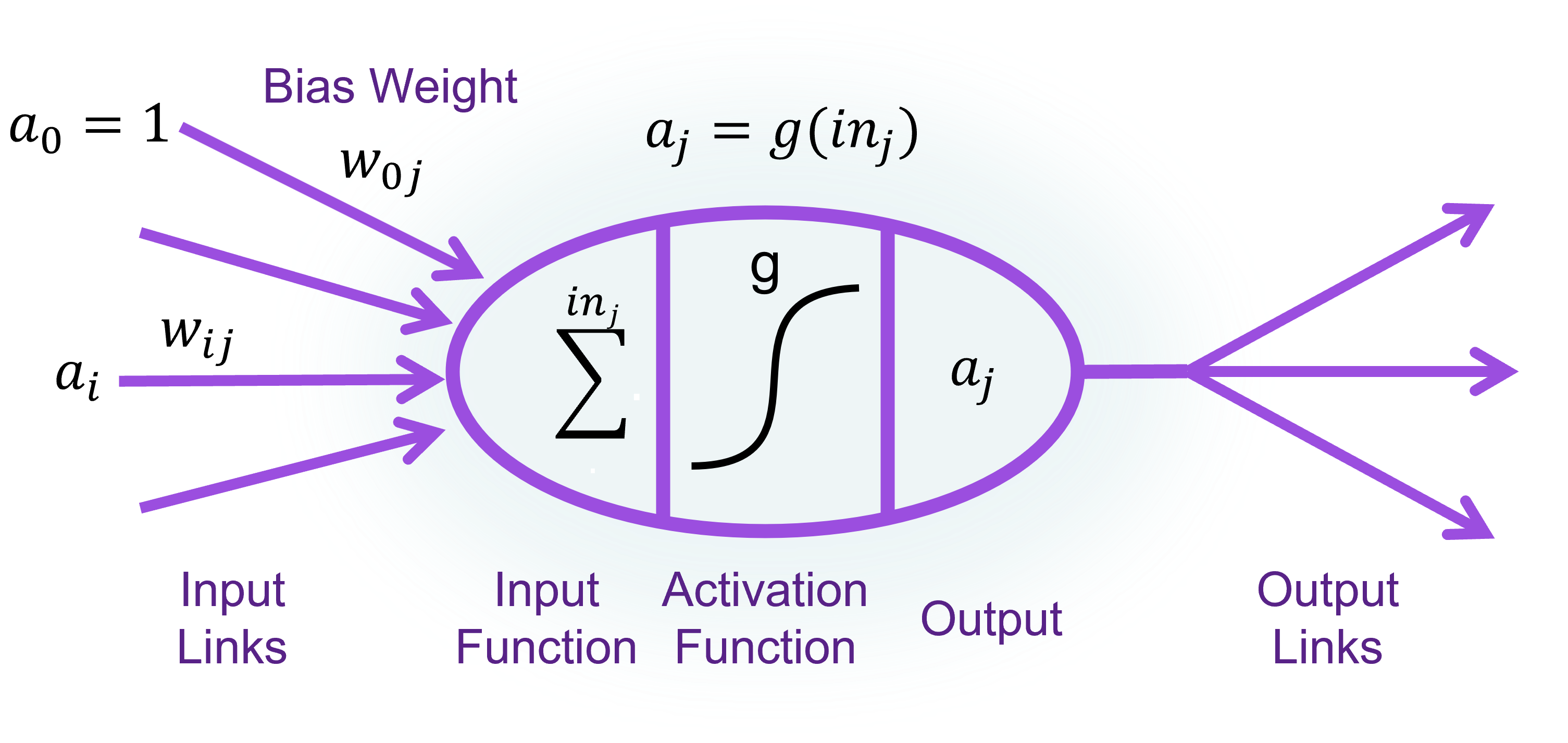
  • a collection of units (neurons) connected together
  • The properties of the network are determined by its topology and the properties of the neurons.
  • Roughly speaking, the neuron fires when a linear combination of its inputs exceeds some (hard or soft) threshold.

Simple Neuron

  • inj=i=0nwijaiin_j = \sum_{i=0}^{n} w_{ij}a_i
  • outj=g(inj)out_j = g(in_j)
  • aj=g(i=0nwijai)a_j = g(\sum_{i=0}^{n} w_{ij} a_i)

Activation function

ReLU function

ReLU(x)=max(0,x)ReLU(x) = max(0, x)

  • an abbreviation for rectified linear unit
  • Commonly used

Softplus function

Softplus(x)=log(1+ex)Softplus(x) = \log(1 + e^x)

  • A smooth version of the ReLU function

Logistic or Sigmoid function

Logistic(x)=11+exLogistic(x) = \frac{1}{1 + e^{-x}}

  • Non-linear, can represent a nonlinear function

Tanh function

tanh(x)=e2x1e2x+1tanh(x) = \frac{e^{2x} -1}{e^{2x} + 1}

Topology of a neural network

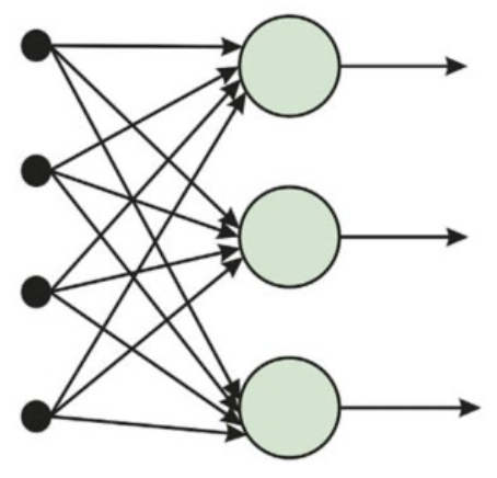
  • Feed-forward network (FFN):
    • Every node receives inputs from "upstream" nodes and delivers output to "downstream" nodes.
    • There are no loops.
    • FFN represents a function of its current inputs, thus it has no internal state other than the weights themselves.
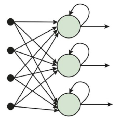
  • Recurrent Network (RNN):
    • A recurrent network feeds its outputs back into its own inputs.
    • In a recurrent network, the neuron values can eventually settle down, keep cycling, or behave unpredictably.
    • can support short-term memory
FFNRNN
FFNRNN

Training Process

  • Go through each training sample.
  • If correctly classified → do nothing.
  • If misclassified → update the weights:
  • wiwi+α(yy^)xiw_i \leftarrow w_i + \alpha(y - \hat{y})x_i

Perceptron for Binary Classification

  • A perceptron separates data into two classes with a hyperplane.
  • if wx01w \cdot x \geq 0 \rightarrow 1
  • if wx00w \cdot x \le 0 \rightarrow 0

Learning Rules

AspectPerceptron Learning RuleGradient Descent (with Sigmoid)
Activation functionHard threshold (계단 함수)
Threshold(z)=1  if  z0,  0  otherwiseThreshold(z) = 1 \; \text{if} \; z \ge 0,\; 0 \; \text{otherwise}
Sigmoid (연속 함수)
hw(x)=11+ewxh_w(x) = \frac{1}{1+e^{-w \cdot x}}
Output0 또는 10과 1 사이의 실수 값
Loss function없음 (틀리면 조정, 맞으면 유지)
규칙 기반 학습
L=(yhw(x))2L = (y - h_w(x))^2 (L2 loss)
또는 Cross-Entropy (실무에서 자주 사용)
Update rule틀렸을 때만:
ww+α(yhw(x))xw \leftarrow w + \alpha (y - h_w(x))x
경사하강법:
ww+α(yhw(x))hw(x)(1hw(x))xw \leftarrow w + \alpha (y - h_w(x)) \cdot h_w(x)(1-h_w(x)) \cdot x
Why derivative?Hard threshold는 미분 불가능 → 단순 규칙 사용Sigmoid는 연속적이고 미분 가능 → Loss 함수의 기울기(gradient)를 따라 업데이트.
여기서 hw(x)(1hw(x))h_w(x)(1-h_w(x)) 항은 sigmoid의 도함수에서 나온 것.
Interpretation틀리면 정답 방향으로 한 걸음 이동Loss가 줄어드는 방향으로 점진적으로 이동

Feadforward NN, FNN

  • a multilayer perceptron network
  • one input layer, N hidden layers, N >= 1, and one output layer.
  • Except for the input layer, each layer has a same activation function g.
  • The final output is represented by a vector function of inputs and weights.
  • If it has three layers, Shallow Neural Network, otherwise Deep Neural Network.

Traning a FNN

  • Forward
    • Activation passing from the input layer to the output layer
    • Calculate the output
  • Backward
    • Errors propagating backward from the output layer to the input layer
    • Update weights

Forward phase

  • Activation of each node is computed in two steps:

    1. Weighted sum (in): sum of activations from the previous layer, multiplied by weights.
    2. Apply activation function g: pass the weighted sum through g to produce the node's activation.
  • Process: propagate activations layer by layer towards the output layer.

  • Output value (example with 2 layers):

    • hw(x)=g(2)(W(2)g(1)(W(1)x))h_w(x) = g^{(2)}\big(W^{(2)} g^{(1)}(W^{(1)} x)\big)

Backward phase

  • Loss function: choose squared error loss (L2)
    • L2(y,y^)=(yy^)2L_2(y, \hat{y}) = (y - \hat{y})^2
  • Prediction:
    • y^=hw(x)\hat{y} = h_w(x)
  • Gradient descent: compute gradient of the loss with respect to weights, then update weights along the negative gradient direction.
    • wi,jwi,jαgradientwi,jw_{i,j} \leftarrow w_{i,j} - \alpha \cdot gradient_{w_{i,j}}
  • Example: sigmoid activation:
    • y^=11+ewx\hat{y} = \frac{1}{1 + e^{-w \cdot x}}
    • Gradient of the loss:
      • gradientwi,j=wi,jLoss(hw)=2(yhw(x))(wi,jhw(x))gradient_{w_{i,j}} = \frac{\partial}{\partial w_{i,j}} Loss(h_w) = 2 (y - h_w(x)) \cdot \Big(- \frac{\partial}{\partial w_{i,j}} h_w(x)\Big)
    • Chain rule applied:
      • g(f(x))x=g(f(x))f(x)\frac{\partial g(f(x))}{\partial x} = g'(f(x)) \cdot f'(x)
  • Example: Gradient derivation for sigmoid
    • Weighted input
      • WX=w1,3x1+w2,3x2+w0,3x0W \cdot X = w_{1,3}x_1 + w_{2,3}x_2 + w_{0,3}x_0
      • (where x0=1x_0 = 1 for the bias)
    • Gradient of the loss
      • gradientwi,j=wi,jLoss(hw)=2(yhw(x))(wi,jhw(x))gradient_{w_{i,j}} = \frac{\partial}{\partial w_{i,j}} Loss(h_w) = 2 (y - h_w(x)) \cdot \Big(-\frac{\partial}{\partial w_{i,j}} h_w(x)\Big)
    • Derivative of sigmoid output
      • wi,jhw(x)=hw(x)(1hw(x))wi,j(WX)\frac{\partial}{\partial w_{i,j}} h_w(x) = h_w(x)(1 - h_w(x)) \cdot \frac{\partial}{\partial w_{i,j}} (W \cdot X)
        • wi,j(11+eWX)\frac{\partial}{\partial w_{i,j}} \left( \frac{1}{1 + e^{-W X}} \right)
        • =(11+eWX)(111+eWX)wi,j(WX)= \left( \frac{1}{1 + e^{-W X}} \right) \left(1 - \frac{1}{1 + e^{-W X}} \right) \cdot \frac{\partial}{\partial w_{i,j}} (W X)
        • =hw(x)(1hw(x))wi,j(WX)= h_w(x) \big(1 - h_w(x)\big) \cdot \frac{\partial}{\partial w_{i,j}} (W X)
    • Derivative of weighted input
      • w0,3(WX)=x0=1\frac{\partial}{\partial w_{0,3}}(W \cdot X) = x_0 = 1
      • w1,3(WX)=x1\frac{\partial}{\partial w_{1,3}}(W \cdot X) = x_1
      • w2,3(WX)=x2\frac{\partial}{\partial w_{2,3}}(W \cdot X) = x_2
    • Weight update rule
      • General form: wi,jwi,jαgradientwi,jw_{i,j} \leftarrow w_{i,j} - \alpha \cdot gradient_{w_{i,j}}
      • w0,3w0,3+α(yhw(x))hw(x)(1hw(x))w_{0,3} \leftarrow w_{0,3} + \alpha (y - h_w(x)) h_w(x)(1 - h_w(x))
      • w1,3w1,3+α(yhw(x))hw(x)(1hw(x))x1w_{1,3} \leftarrow w_{1,3} + \alpha (y - h_w(x)) h_w(x)(1 - h_w(x)) x_1
      • w2,3w2,3+α(yhw(x))hw(x)(1hw(x))x2w_{2,3} \leftarrow w_{2,3} + \alpha (y - h_w(x)) h_w(x)(1 - h_w(x)) x_2

Backward phase Steps

  1. Select a loss function
    • For example, squared error loss:
    • L(y,y^)=(yy^)2,y^=hw(x)L(y, \hat{y}) = (y - \hat{y})^2, \quad \hat{y} = h_w(x)
  2. Choose an activation function
    • Suppose we use a sigmoid:
    • hw(x)=11+eWXh_w(x) = \frac{1}{1 + e^{-W \cdot X}}
  3. Calculate the error at the output node
    • The delta (error term) at the output is
    • Δout=2(y^y)g(inout)\Delta_{out} = 2(\hat{y} - y) \cdot g'(in_{out})
  4. Calculate the error at hidden nodes
    • A hidden unit may connect to multiple nodes in the next layer.
    • Therefore, its error is the weighted sum of all deltas it feeds into, scaled by its own derivative:
    • Δi=g(ini)jwi,jΔj \Delta_i = g'(in_i) \sum_j w_{i,j} \Delta_j
    • The summation appears because the hidden node's output influences several downstream nodes, and all those error signals must be aggregated.
  5. Update the weights with gradient descent
    • The gradient with respect to weight wi,jw_{i,j} is simply the input times the delta:
    • Lwi,j=aiΔj\frac{\partial L}{\partial w_{i,j}} = a_i \Delta_j
    • Update rule:
    • wi,jwi,jαaiΔjw_{i,j} \leftarrow w_{i,j} - \alpha \, a_i \Delta_j

Vanishing gradient

  • The error signal are extinguished altogher as they are propagated back through the network
  • In deep feedforward networks with sigmoid/tanh, repeated multiplication of small derivatives (0<g(z)<10 < g'(z) < 1) during backpropagation causes the gradient to vanish.

Optimizer

  • Training a neural network consists of modifying the network's parameters, minimizing the loss function on the training set.
  • any kind of optimization algorithm could be used.
  • modern neural networks are almost always trained with some variant of stochastic gradient descent (SGD). Adam Optimizer
  • The optimiser is specified in the compilation step with tensorflow.

Recurrent NN, RNN

  • units may take as input a value computed from their own output at an earlier step in the computation.
  • have internal state, or memory: inputs received at earlier time steps affect the RNN's response to the current input.
  • be used to perform more general computations.
    • to analyze sequential data in which a new input vector xtx_t arrives at each time step
  • Markov assumption: the hidden state ztz_t of the network suffices to capture the information from all previous inputs.
    • zt=f(zt1,xt)z_t = f(z_{t-1}, x_t)
    • Once trained, this function represents a time-homogeneous process
    • The same update rule fwf_w applies at every time step, regardless of whether it’s the first input or the hundredth.
  • RNNs are designed for sequential data.
  • a hidden state that captures information from previous steps.
  • suffer from vanishing/exploding gradients.
  • Good for short-term dependencies.

Backpropagtion Through Time, BPTT

  • gradient expression is recursive.
    • ztwz,z\frac{\partial z_t}{\partial w_{z,z}}
    • =wz,zgz(inz,t)= \frac{\partial}{\partial w_{z,z}} g_z(in_{z,t})
    • =gz(inz,t)inz,twz,z= g_z'(in_{z,t}) \frac{\partial in_{z,t}}{\partial w_{z,z}}
    • =gz(inz,t)wz,z(wz,zzt1+wx,zxt+w0,z)= g_z'(in_{z,t}) \frac{\partial}{\partial w_{z,z}} (w_{z,z} z_{t-1} + w_{x,z} x_t + w_{0,z})
    • =gz(inz,t)(zt1+wz,zzt1wz,z)= g_z'(in_{z,t}) \left( z_{t-1} + w_{z,z} \frac{\partial z_{t-1}}{\partial w_{z,z}} \right)
      • ztWz,z\frac{\partial z_t}{\partial W_{z,z}} includes zt1Wz,z\frac{\partial z_{t-1}}{\partial W_{z,z}}
  • the gradient with run time being linear in the size of the network
  • handled automatically by deep learning software systems.
  • Iterating the recursion shows that the gradient at time TT includes a term proportional to:
    • wz,zt=1Tgz(inz,t)w_{z,z} \prod_{t=1}^{T} g'_z(in_{z,t})
  • Since for sigmoid, tanh, and ReLU we have g1g' \leq 1, if wz,z<1w_{z,z} < 1 the RNN will suffer from the vanishing gradient problem.
  • If wz,z>1w_{z,z} > 1, we may encounter the exploding gradient problem.

Long Short-Term Memory, LSTM

  • memory cell is essentially copied from time step to time step.
  • New information enters the memory by adding updates.
    • the gradient expressions do not accumulate multiplicatively over time.
  • include gating units: vectors control the flow of information in the LSTM, elementwise multiplication of the corresponding information vector.
  • a type of RNN designed to overcome vanishing gradient.
  • use gates (input, forget, output) to control information flow.
  • Capable of learning long-term dependencies.
  • Widely used in NLP, speech recognition, and time series forecasting.

Gates in LSTM

  • Forget gate: decides what information to discard from the cell state.
  • Input gate: decides what new information to store in the cell state.
  • Output gate: decides what information to output from the cell state.
    • similar role to the hidden state in basic RNNs.
  • Update equations:
    • ft=σ(Wx,fxt+Wz,fzt1)f_t = \sigma(W_{x,f}x_t + W_{z,f}z_{t-1})
      • Decides which parts of the previous cell state ct1c_{t-1} should be kept or discarded.
    • it=σ(Wx,ixt+Wz,izt1)i_t = \sigma(W_{x,i}x_t + W_{z,i}z_{t-1})
      • Determines how much of the new information from the current input xtx_t and the previous hidden state zt1z_{t-1} should be added.
    • ot=σ(Wx,oxt+Wz,ozt1)o_t = \sigma(W_{x,o}x_t + W_{z,o}z_{t-1})
      • Controls which parts of the current cell state ctc_t are exposed as the hidden state ztz_t.
    • ct=ct1ft+ittanh(Wx,Cxt+Wz,Czt1)c_t = c_{t-1} \odot f_t + i_t \odot \text{tanh}(W_{x,C}x_t + W_{z,C}z_{t-1})
      • Cell state update
      • Past information (ct1c_{t-1}) is partially retained through the forget gate.
      • New information is added through the input gate and tanh\tanh.
      • Thus, ctc_t serves as the long-term memory of the LSTM.
    • zt=ottanh(ct)z_t = o_t \odot \text{tanh}(c_t)
      • Hidden state update
      • The cell state is normalized with tanh(ct)\tanh(c_t) and filtered by the output gate.
      • ztz_t is the hidden state passed forward to the next time step.

Gated Recurrent Unit, GRU

  • Variant of RNN with gating mechanisms.
  • Designed to capture long-term dependencies without complex architecture.
  • a simpler alternative to LSTMs. (lightweight, effective RNN variant)
  • Captures temporal dependencies (short & long).
  • Combine input and forget gates into a single update gate.
  • Require fewer parameters than LSTM, making them faster to train.
  • Perform comparably to LSTMs in many tasks.
  • Prevents vanishing gradient.
  • Good balance between complexity & performance.
  • Excels in time series forecasting tasks.
  • Widely used in finance, energy and IoT.

Gates in GRU

  • Update gate (z): decides how much past information to keep
  • Reset Gate (r): decides how much past information to forget
  • Candidate hidden state (h~\tilde{h}): potential new memory
  • Final hidden state (hh): weighted combination of old and new information.

GRU Workflow

  • Reset gate (rr)
    • Controls how much of the previous hidden state should be "forgotten."
    • A small value means most of the past memory is erased, while a large value means much of it is retained.
  • Update gate (zz)
    • Acts as a switch to decide whether to keep the previous state hprevh_{prev} or replace it with the new candidate h~\tilde{h}.
    • If z=1z=1, the past is fully kept; if z=0z=0, it is completely replaced by the new candidate.
  • Candidate state (h~\tilde{h})
    • Combines the current input xtx_t with the reset-gated previous hidden state to generate the "candidate" new information.
  • Final hidden state (hh)
    • Blends the past and the candidate using the update gate zz.
    • If zz is large → the past memory dominates.
    • If zz is small → the new candidate dominates.
  • h=(1z)h~+zhprevh=(1−z)\tilde{h}+zh_{prev}

Comparison: RNN vs LSTM vs GRU

AttributeRNNLSTMGRU
ArchitectureSimple, hidden stateComplex, memory cell + 3 gatesSimplified, 2 gates (update/reset)
Information FlowStored in hidden stateControlled by gatesControlled by merged gates
Long-term DependencyWeak (vanishing gradient)Strong (gates solve vanishing gradient)Strong (gates solve vanishing gradient)
Short-term DependencyStrongStrongStrong
Number of ParametersFewManyFewer than LSTM
Training SpeedFastSlowFast
PerformanceGood for short-termGood for long-termEfficient, similar to LSTM
Application AreasSimple time series, basic NLPNLP, speech, time series forecastingFinance, IoT, energy, time series
Vanishing GradientYesNoNo
Typical Use CasesText generation, simple predictionTranslation, speech recognitionTime series prediction, sensor data
SimplicityVery simple, rarely usedMore complex, expressive (3 gates)Simpler than LSTM, fewer parameters
ExpressivenessLimited, struggles with long-termHigh, handles very complex sequencesModerate, good for moderate data size
Training EfficiencyFast, but limitedSlower, better for complex dataFast, efficient, similar performance
Trade-offSimple but weak for long-termCapacity for complex, long sequencesSimplicity vs. capacity

Open X-Embodiment review

· 5 min read

RT-X

  • RT-X trains generalist robot policies by co-training RT-1/RT-2 on an X-embodiment mix of multi-robot, multi-task data, enabling efficient adaptation to new robots, tasks, and environments.
  • It standardizes 1M+ trajectories from 22 embodiments into the Open X-Embodiment (RLDS/tfrecord) repository, unifying observations and 7-DoF actions via coarse alignment.
  • Experiments show strong positive transfer and emergent skills (≈3× with RT-2-X on cross-robot tasks); performance scales with model capacity, short image histories, and web pretraining, while sensing/actuation diversity and frame alignment remain open problems.

RT-X Architecture

Motivation

  • Seeks a generalist X-robot policy that can be efficiently adapted to new robots, tasks, and environments.
  • Mirrors a trend from CV/NLP where general-purpose, web-scale pretrained models outperform narrow, task-specific models.
  • Robotics lacks comparably large, diverse interaction datasets, making direct transfer of these lessons challenging.

Objectives

  1. Positive transfer: Test whether co-training on data from many robots improves performance on each training domain.
  2. Ecosystem building: Organize large robotic datasets to enable future X-embodiment research.

Core Approach

  • Train RT-1 and RT-2 on data from 9 different manipulators, producing RT-X variants that outperform policies trained only on the evaluation domain and show better generalization and new capabilities.

What’s Different From Prior Transfer Methods

  • Many prior works reduce the embodiment gap via specialized mechanisms (shared action spaces, representation learning objectives, policy adaptation using embodiment metadata, decoupled robot/environment representations, domain translation).
  • RT-X directly trains on X-embodiment data without explicit gap-reduction machinery and still observes positive transfer.

Dataset & Format (Open X-Embodiment)

  • 1M+ real robot trajectories, 22 embodiments (single-arm, bimanual, quadrupeds), pooled from 60 datasets / 34 labs, standardized for easy use.
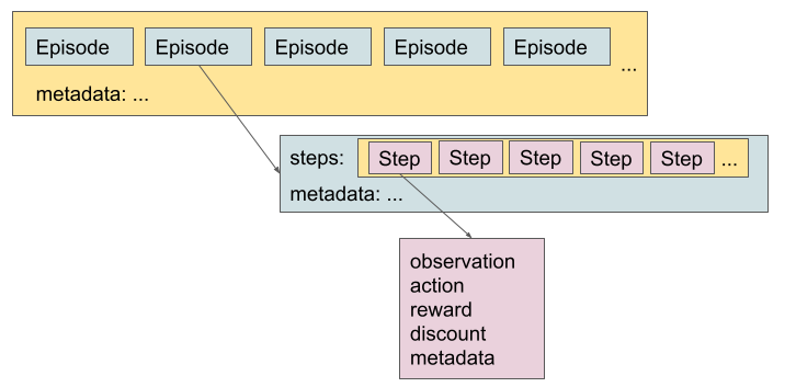
  • Uses RLDS (serialized tfrecord), supporting varied action spaces and input modalities (RGB, depth, point clouds), and efficient parallel loading across major DL frameworks.
  • Language annotations are leveraged; PaLM is used to extract objects/behaviors from instructions.

RLDS

Data Format Consolidation (Coarse Alignment)

  • Observations: History of recent images + language instruction. One canonical camera view per dataset is resized to a common resolution.
  • Actions: Convert original controls to a 7-DoF end-effector vector (x, y, z, roll, pitch, yaw, gripper or their rates). Actions are normalized before discretization; outputs are de-normalized per embodiment.
  • Deliberate non-alignment: Camera poses/properties are not standardized; action frame alignment across datasets is not enforced. The same action vector may cause different motions on different robots (absolute/relative, position/velocity allowed).

Policy Architectures

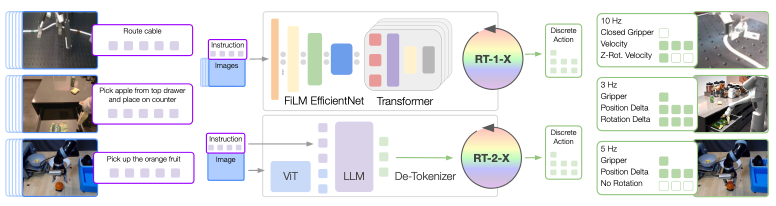
  • RT-1 (≈35M params): Transformer for control. Inputs: 15-frame image history + natural-language instruction.
    • Vision via ImageNet-pretrained EfficientNet; language via USE embedding.
    • Fuse via FiLM → 81 vision–language tokens → decoder-only Transformer outputs tokenized actions.
  • RT-2 (VLA family): Internet-scale VLM co-fine-tuned to output action as text tokens (e.g., 1 128 91 241 5 101 127).
    • Any pretrained VLM can be adapted; this work uses RT-2–PaLI-X (ViT backbone + UL2 LM; primarily pretrained on WebLI).

Training Setup

  • Robotics data mixture: Data from 9 manipulators (a union of multiple well-known robotics datasets).
  • Loss: Standard categorical cross-entropy over tokenized actions.
  • Regimes:
    • RT-1-X: Trained solely on the robotics mixture.
    • RT-2-X: Co-fine-tuned on a ~1:1 mix of original VLM data and the robotics mixture.

Experimental Questions

  1. Does X-embodiment co-training improve in-domain performance (positive transfer)?
  2. Does it improve generalization to unseen tasks?
  3. How do model size, architecture, and dataset composition influence performance/generalization?

Key Results

  • Small-scale domains: RT-1-X outperforms the Original Method (the authors’ per-dataset baselines) on 4/5 datasets with a large average gain → limited data domains benefit greatly from X-embodiment co-training.
  • Large-scale domains:
    • RT-1-X does not beat an RT-1 trained only on the embodiment-specific large dataset (suggests underfitting for this class).
    • RT-2-X (larger capacity) outperforms both Original Method and RT-1 → X-robot training helps even in data-rich regimes when using sufficient capacity.

Generalization & Emergent Skills

  • Unseen objects/backgrounds/environments: RT-2 and RT-2-X perform on par (VLM backbone already strong here).
  • Emergent skills (transfer across robots): On Google Robot tasks that do not appear in RT-2’s dataset but exist in Bridge (for WidowX), RT-2-X ≈ 3× RT-2.
    • Removing Bridge from RT-2-X training significantly reduces hold-out performance → skills likely transferred from WidowX data.

Design Insights (Ablations)

  • Short image history notably improves generalization.
  • Web pretraining is critical for large models’ high performance.
  • Model capacity matters: 55B model succeeds more than 5B on emergent skills → greater capacity ⇒ greater cross-dataset transfer.
  • Co-fine-tuning vs. fine-tuning: Similar performance in this study (attributed to the greater diversity of robotics data in RT-2-X vs. prior works).

Limitations (Open Problems)

  • Does not cover robots with very different sensing/actuation modalities.
  • Does not study generalization to new robots nor define a decision criterion for when positive transfer will occur.
  • Camera pose/properties and control frame remain unaligned; a deliberate but still challenging domain gap to address in future work.

Ref

  • O’Neill, A., Rehman, A., Maddukuri, A., Gupta, A., Padalkar, A., Lee, A., Pooley, A., Gupta, A., Mandlekar, A., & Jain, A. (2024). Open x-embodiment: Robotic learning datasets and rt-x models: Open x-embodiment collaboration 0. 2024 IEEE International Conference on Robotics and Automation (ICRA).

FSD +006

· 4 min read

OOP vs Procedural Programming

OOP

  • a programming paradigm built around the concept of objects, which contain data and code to manipulate data.
  • The idea to model real-world entities and their interactions.
  • Global Data (fields) are enclosed in the objects.
  • Program components/tasks are easily divided across the development team / Requires more planning and design preparation
  • Easier to manage and maintain dependencies between objects / OOP programs are much larger and complex
  • Objects export the interface and hide the implementation and data / Tend to use more memory and GPU
  • Code is highly reusable and easy to scale and distribute / Making changes in one class potentially impact others, which can complicate the development of the code.

Procedural Programming

  • the concept of procedure calls by structuring the program around procedures. (or functions/subroutines)
  • a sequential manner unless directed otherwise.
  • Global data (elements) is exposed to all the functions.
  • Easier to compile and interpret / Difficult to scale or extend
  • Straightforward and simpler to code / Dependencies between elements are unclear and not well-structured.
  • Less memory requirements / Data is exposed and insecure due to its exposure across the whole program
  • Easy to track the program flow / Hard to divide the work among programmers in a team.

Classes

  • A class is a template/blueprint used to create objects
javapython
a pure OOP languagesupports OOP
code must be written in classesclasses are optional
executable class must have main()scripts run without including a class
Encapsulation can be enforced by declaring fields as privatefields (global variables) are public by default
Visibility is managed through access modifiersN/A ("_" to identify private data attributes, but still accessible)
class <class-name> (<extend - superclass>):
<variable-name> = <value> #Class fields - data members

def __init(self, <parameters>): #class constructor - object sbuilder
<code>

<method-name> (self, <parameters>): #methods
<code>

Classes Py

KeywordsFunctions
class__init__()
self: keyword used to refer to object propertiesdel: the function is used to delete an object
pass: keyword used to occupy no-code placement in a function__str__(): The function is used to return string representation of instances
cls: keyword used to refer to class propertiessuper(): the function is used call a parent method in a child class
  • Accessors: functions (with no parameters) in a Python class that provide access to the data attributes of an object.
    • known as getter methods, are named starting with the verb get, followed by the field name, which should start with an uppercase letter.
  • Mutators: procedures (with parameter) in a Python class that enable the developer to modify the values of object attributes.
    • known as setter methods, are named starting with the verb set, followed by the field name, which should start with an uppercase letter.
def get<Variable> ():
return self.<field>

def set<Variable> (self, value):
self.<field> = value

Classes Java

public class Bank {
private Customer customer;
private String branch;

public Bank() {
customer = new Customer();
}

public Bank(String name) {
this();
this.branch = name;
}

public boolean find(Bank bank) {
return this.branch.equals(bank.branch);
}
}

Packages

Packages Java

  • used to group related classes
  • like folders containing files (classes)
  • either Java defined or user-defined
  • used to write maintainable and portable code and to avoid class name conflicts.

Modules Py

  • used to grou prelated functio nand classes together
  • normal Python scripts that are used into other scripts
  • either Python defined or user-defined
  • used to write maintainable and portable code to improve reusability

π0 Review

· 4 min read

π0

Problem & Motivation

  • Achieving real-world generality in robot learning is blocked by data scarcity, generalization, and robustness limits.
  • Human intelligence most outpaces machines in versatility—solving diverse, physically situated tasks under constraints, language commands, and perturbations.
  • In NLP/CV, foundation models pre-trained on diverse multi-task data, then fine-tuned (aligned) on curated datasets, outperform narrow specialists; the same paradigm is hypothesized for robotics.

Core Proposal

  • A novel flow-matching architecture built on a pre-trained Vision-Language Model (VLM) to inherit Internet-scale semantics.
  • Further training adds robot actions, turning the model into a Vision-Language-Action (VLA) policy.
  • Use cross-embodiment training to combine data from many robot types (single/dual-arm, mobile), despite differing configuration/action spaces.
  • Employ action chunking + flow matching (diffusion variant) to model complex, continuous, high-frequency actions.
  • Introduce an Action Expert (separate weights for action/state tokens), akin to a Mixture-of-Experts, augmenting the standard VLM.

Training Recipe (Pre- vs Post-Training)

  • Pre-training on highly diverse data builds broad, general physical abilities.
  • Post-training on curated, task-specific data instills fluent, efficient strategies.
  • Rationale: high-quality-only training lacks recovery behaviors; low-quality-only training lacks efficiency/robustness; combining both yields desired behavior.

Data & Backbone

  • ~10,000 hours of demonstrations + the OXE dataset; data spans 7 robot configurations and 68 tasks.
  • VLM backbone initialized from PaliGemma (3B); add ~300M parameters for the action expert (total ~3.3B).
  • Pre-training mixture: weighted combination of internal datasets + full OXE; n^0.43 weighting to down-weight overrepresented task-robot pairs.
  • Unify interfaces: zero-pad qt/at to the largest robot dimension (18); mask missing image slots; late-fusion encoders map images/states to the same token space as language.

Modeling Details

  • Conditional flow matching models the continuous distribution over action chunks.
  • Train with a diffusion-style loss on individual sequence elements (instead of cross-entropy), with separate weights for diffusion-related tokens.
  • Flow path uses a linear-Gaussian schedule; sample noisy actions with ε∼N(0, I); predict denoising vector field; Euler integration from τ=0→1 at inference.
  • Efficient inference by caching K/V for the observation prefix; action tokens recomputed per integration step.

High-Level Language Policy

  • Because the policy consumes language, a high-level VLM can decompose tasks (e.g., bussing) into intermediate language subgoals (SayCan-style planning), improving performance on complex, temporally extended tasks.

Evaluation Setup & Baselines

  • Out-of-box (direct prompting), fine-tuning on downstream tasks, and with high-level VLM providing intermediate commands.
  • Compare against OpenVLA (7B, autoregressive discretization; no action chunks/high-frequency control) and Octo (93M; diffusion), trained on the same mixture.
  • Include a compute-parity π0 (160k steps vs 700k) and a π0-small variant (no VLM init).

Key Results

  • Out-of-box: π0 outperforms all baselines; even compute-parity π0 beats OpenVLA/Octo; π0-small still surpasses them—highlighting the benefits of expressive architectures + diffusion/flow matching + VLM pre-training.
  • Language following: π0 clearly exceeds π0-small across conditions:
    • π0-flat: only overall task command.
    • π0-human: human-provided intermediate steps.
    • π0-HL: high-level VLM-provided steps (fully autonomous).
    • Better language-following accuracy directly translates into stronger autonomous performance with high-level guidance.
  • New dexterous tasks (e.g., bowls stacking, towel folding, microwave, drawer items, paper towel replacement):
    • Fine-tuned π0 generally outperforms OpenVLA, Octo, and small-data methods ACT / Diffusion Policy.
    • Pre-training helps most when tasks resemble pre-training data; pretrained π0 often beats from-scratch by up to .
  • Complex multi-stage tasks (laundry folding, table bussing, box building, to-go box, eggs):
    • π0 solves many tasks; full pre-training + fine-tuning performs best.
    • Gains from pre-training are especially large on harder tasks; absolute performance varies with task difficulty and pre-training coverage.

Takeaways & Limitations

  • π0 mirrors LLM training: pre-train for knowledge, post-train for alignment (instruction-following and execution).
  • Limitations/open questions:
    • Optimal composition/weighting of pre-training data remains unclear.
    • Not all tasks work reliably; difficult to predict how much/what kind of data is needed for near-perfect performance.
    • Uncertain positive transfer across very diverse tasks/robots and to distinct domains (e.g., driving, navigation, legged locomotion).

Ref

  • Black, K., Brown, N., Driess, D., Esmail, A., Equi, M., Finn, C., Fusai, N., Groom, L., Hausman, K., Ichter, B., Jakubczak, S., Jones, T., Ke, L., Levine, S., Li‑Bell, A., Mothukuri, M., Nair, S., Pertsch, K., Shi, L. X, … Zhilinsky, U. (2025, June 21). π₀: A vision‑language‑action flow model for general robot control Robotics: Science and Systems (RSS), Los Angeles, CA, United States. https://roboticsconference.org/program/papers/10/

Vima Review

· 2 min read

VIMA

  • Unified Multimodal Prompts: Reformulates diverse robot tasks (language, images, video) into a single sequence modeling problem.
  • Object-Centric Tokenization: Uses object-level tokens (Mask R-CNN + ViT) instead of raw pixels, improving data efficiency and semantic generalization.
  • Cross-Attention Conditioning: Conditions the policy on prompts via cross-attention, maintaining strong zero-shot performance even with small models or novel tasks.

Motivation

  • Robot task specification comes in many forms: one-shot demonstrations, language instructions, and visual goals.
  • Traditionally, each task required distinct architectures and pipelines, leading to siloed systems with poor generalization.

VIMA Architecture

Key Contributions

  1. Multimodal Prompting

    • A novel formulation that unifies diverse robot manipulation tasks into a sequence modeling problem.
    • Prompts are defined as interleaved sequences of text and images, enabling flexibility across task formats.
  2. VIMA-BENCH

    • A large-scale benchmark with 17 tasks across six categories (object manipulation, goal reaching, novel concept grounding, video imitation, constraint satisfaction, visual reasoning).
    • Provides 650K expert trajectories and a four-level evaluation protocol for systematic generalization.
  3. VIMA Agent

    • A transformer-based visuomotor agent with encoder-decoder architecture and object-centric design.
    • Encodes prompts with a pre-trained T5 model, parses images into object tokens via Mask R-CNN + ViT, and decodes actions autoregressively using cross-attention.

Design Insights

  • Object-Centric Representation: Passing variable-length object token sequences directly to the controller is more effective than pixel-based tokenization.
  • Cross-Attention Conditioning: Stronger prompt focus and efficiency compared to simple concatenation (e.g., GPT-style).
  • Robustness: Minimal degradation under distractors or corrupted prompts, aided by T5 backbone and object augmentation.

Results

  • Performance:

    • Outperforms baselines (VIMA-Gato, VIMA-Flamingo, VIMA-GPT) by up to 2.9× success rate in hardest zero-shot generalization.
    • With 10× less training data, still 2.7× better than best competitor.
  • Scaling:

    • Sample-efficient: with just 1% of data, matches baselines trained with 10× more.
    • Generalization holds across L1–L4 evaluation, with smaller regression than alternatives.

Conclusion

VIMA demonstrates that multimodal prompting is a powerful unifying framework for robot learning.
It achieves strong scalability, data efficiency, and generalization, establishing a solid starting point for future generalist robot agents.

Ref

  • Jiang, Y., Gupta, A., Zhang, Z., Wang, G., Dou, Y., Chen, Y., Fei-Fei, L., Anandkumar, A., Zhu, Y., & Fan, L. (2023). VIMA: Robot Manipulation with Multimodal Prompts Proceedings of the 40th International Conference on Machine Learning, Proceedings of Machine Learning Research. https://proceedings.mlr.press/v202/jiang23b.html

RoboFlamingo Review

· 2 min read

RoboFlamingo

  • RoboFlamingo decouples vision-language understanding and control, using OpenFlamingo for perception and a lightweight policy head for sequential decision-making.
  • Unlike prior VLM-based approaches, it requires only small-scale imitation fine-tuning on language-conditioned manipulation data, without large-scale co-fine-tuning.
  • This design enables data-efficient, zero-shot generalizable, and deployable robot manipulation policies on modest compute resources.

Key Idea

  • Proposes RoboFlamingo, a simple framework to adapt existing VLMs for robotic manipulation with lightweight fine-tuning.
  • Built on OpenFlamingo, decoupling vision-language understanding from decision-making.
  • Pre-trained VLM handles language and visual comprehension, while a dedicated policy head models sequential history.
  • Fine-tuned only on language-conditioned manipulation datasets using imitation learning.

Advantages

  • Requires only a small amount of demonstrations to adapt to downstream manipulation tasks.
  • Provides open-loop control capability → deployable on low-performance platforms.
  • Can be trained/evaluated on a single GPU server, making it a cost-effective and accessible solution.

Benchmarks

  • Evaluated on CALVIN benchmark (34 tasks, 1000 instruction chains).
  • RoboFlamingo achieves 2× performance improvements over previous state-of-the-art methods.

Performance

  • Imitation Learning: Outperforms all baselines across all metrics.
  • Zero-shot Generalization:
    • Vision: Stronger generalization in ABC→D setting.
    • Language: Robust to GPT-4 generated synonymous instructions.
  • Ablation Studies:
    • Ignoring history (MLP w/o hist) gives worst results.
    • LSTM and GPT-based policy heads perform best (LSTM chosen as default).
    • VL pre-training is crucial for downstream manipulation.
    • Larger VLMs show better data efficiency.
    • Instruction fine-tuning improves both seen and unseen tasks.

Flexibility of Deployment

  • Supports open-loop control by predicting entire action sequences with a single inference → reduces latency and test-time compute.
  • Direct open-loop use without retraining can degrade performance; mitigated with jump-step demonstrations.

Conclusion

  • Demonstrates that pre-trained VLMs enable data efficiency and strong zero-shot generalization in robotic manipulation.
  • RoboFlamingo is presented as an intuitive, efficient, and open solution, with high potential when combined with large-scale real robot data.

Ref

  • Li, X., Liu, M., Zhang, H., Yu, C., Xu, J., Wu, H., Cheang, C., Jing, Y., Zhang, W., & Liu, H. (2024). Vision-language foundation models as effective robot imitators. International Conference on Learning Representations (ICLR 2024), Vienna, Austria.

OpenVLA Review

· 3 min read

OpenVLA

  • OpenVLA is a 7B open-source VLA model built on Llama2 + DINOv2 + SigLIP, trained on 970k demos, achieving stronger generalization and robustness than closed RT-2-X (55B) and outperforming Diffusion Policy.
  • It introduces efficient adaptation via LoRA (1.4% params, 8× compute reduction) and 4-bit quantization (half memory, same accuracy), enabling fine-tuning and inference on consumer GPUs.
  • Limitations remain (single-image input, <90% reliability, limited throughput), but OpenVLA provides the first open, scalable framework for generalist robot policies.

OpenVLA Architecture

Motivation

  • Training robot policies from scratch struggles with robustness and generalization.
  • Fine-tuning vision-language-action (VLA) models offers reusable, generalizable visuomotor policies.
  • Barriers: prior VLAs are closed-source, lack best practices for adaptation, and need server-class hardware.

Model & Training

  • OpenVLA: 7B parameters, open-source.
  • Built on Llama 2 with fused DINOv2 + SigLIP vision encoders.
  • Trained on 970k robot demonstrations from Open-X Embodiment dataset.
  • Represents robot actions as tokens (discretized into 256 bins, replacing unused Llama tokens).
  • Standard next-token prediction objective.

Architecture & Approach

  • End-to-end fine-tuning of VLM to generate robot actions as tokens.
  • Differs from modular methods (e.g., Octo) that stitch separate encoders/decoders.
  • Vision features are obtained by encoding the same input image with both SigLIP and DINOv2, then channel-wise concatenated and passed through an MLP projector. This preserves SigLIP’s semantic alignment with language and DINOv2's spatial reasoning, giving the VLM richer multimodal context for manipulation tasks.
  • Uses Prismatic VLM backbone with multi-resolution features (spatial reasoning + semantics).

Performance

  • Outperforms closed RT-2-X (55B) by +16.5% task success with 7× fewer parameters.
  • Beats Diffusion Policy (from-scratch imitation learning) by +20.4% on multi-task language-grounded settings.
  • Demonstrates robust behaviors (distractor resistance, error recovery).

Efficiency

  • Introduces parameter-efficient fine-tuning:
    • LoRA updates only 1.4% of parameters yet matches full fine-tuning.
    • Can fine-tune on a single A100 GPU in ~10–15 hours (8× compute reduction).
  • Quantization:
    • 4-bit inference matches bfloat16 accuracy while halving memory footprint.
    • Runs at 3Hz on consumer GPUs (e.g., A5000, 16GB).

Evaluations

  • Tested across 29 tasks and multiple robots (WidowX, Google robot, Franka).
  • Strong generalization on:
    • Visual (unseen backgrounds/distractors).
    • Motion (new object positions/orientations).
    • Physical (new object shapes/sizes).
    • Semantic (unseen tasks, instructions).
  • First generalist open-source VLA achieving ≥50% success rate across all tested tasks.

Design Insights

  • Fine-tuning the vision encoder (vs. freezing) crucial for robotic control.
  • Higher image resolution (384px vs. 224px) adds 3× compute without performance gains.
  • Training required 27 epochs, far more than typical VLM runs, to surpass 95% action token accuracy.

Limitations & Future Work

  • Supports only single-image observations (no proprioception, no history).
  • Inference throughput (~6Hz on RTX 4090) insufficient for high-frequency control (e.g., ALOHA at 50Hz).
  • Success rates remain below 90% in challenging tasks.
  • Open questions:
    • Impact of base VLM size on performance.
    • Benefits of co-training with Internet-scale data.
    • Best visual features for VLAs.

Contributions

  1. First open-source generalist VLA with strong performance.
  2. Scalable end-to-end training pipeline (action-as-token).
  3. Demonstrates LoRA + quantization for consumer-grade GPU adaptation.
  4. Provides code, checkpoints, and data curation recipes to support future research.

Ref

  • Kim, M. J., Pertsch, K., Karamcheti, S., Xiao, T., Balakrishna, A., Nair, S., Rafailov, R., Foster, E. P., Sanketi, P. R., Vuong, Q., Kollar, T., Burchfiel, B., Tedrake, R., Sadigh, D., Levine, S., Liang, P., & Finn, C. (2025). OpenVLA: An Open-Source Vision-Language-Action Model Proceedings of The 8th Conference on Robot Learning, Proceedings of Machine Learning Research. https://proceedings.mlr.press/v270/kim25c.html