RL 010

Policy Search Methods

Instead of $V$ and $Q$ functions, we directly estimate the optimal policy.

$\pi^{\theta}(a|s) \approx P(a|s, \theta)$

• Policy was generated directly from the value function (e.g. $\epsilon$-greedy)
• Parameterize the policy directly.
  • Instead of $v(s,w)$ or $\hat{q}(s,a,w)$, we have $\pi^{\theta}(a|s)$
  • Given a particular state $s$, what actions should we take? (What is probability of that particular action?)
  • $\theta$ is a learnable parameter which could be a neural network.

Value-based and Policy-based Methods

• Value-based: Learnt value function, Implicit policy (e.g. $\epsilon$-greedy)
• Policy-based: No value function, Learnt policy.
  • Good convergence properties
  • Effective in high-dimensional or continuous action spaces
    • if it is really continuous and large, it is not efficient as well.
  • Can learn stochastic policies.
  • Sometimes policies are relatively simple, values and models are complex.
  • Typically reaches local optima.
  • Obtained knowledge is specific and does not generalize well.
• Actor-Critic: Learnt value function, Learnt policy.

Policy Gradient Techniques

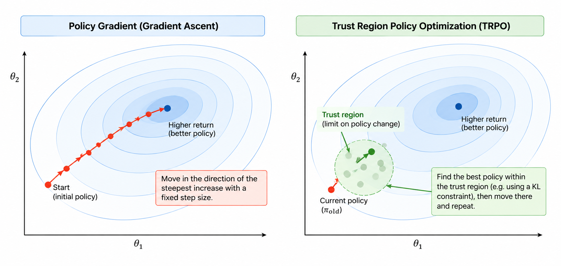
• Trust-Region Based: Optimize the policy in a trust zone (closer circle).

Stochastic policies

Rock-Paper-Scissors

• A deterministic policy is easily exploited
  • Deterministic policy: If we follow a set of action or sequence of actions, we will definitely reach the goal and will always reach teh same location.
• A uniform random policy is optimal policy.

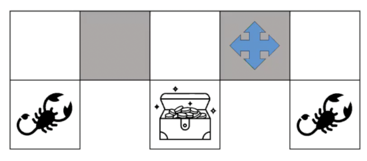
Grid World

$$\phi(s,a) = \big(\underbrace{1 0 1 0}_{walls}, \underbrace{0 1 0 0}_{actions}\big)$$

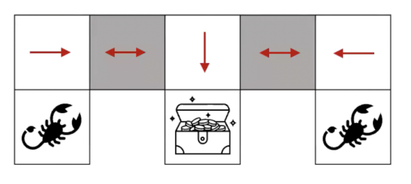
• Agent cannot differentiate between the grey states.
• $\phi(s,a)$ features describing state $s$ and action $a$.
• $\phi(s,E) = (\underbrace{1, 0, 1, 0}_{\text{NESW}}, \underbrace{0, 1, 0, 0}_{\text{NESW}})$ is the North and the South are walls and the agent will move to the East.
• If $\pi(\text{grey}) = W$, then when the agent is in the left grey state, it will move west, get stuck in a loop, and never reach the goal.

• Therefore, an optimal stochastic policy moves randomly $E$ or $W$ in grey states.
  • $\pi_{\theta}(\text{wall to N and S, move E}) = 0.5$
  • $\pi_{\theta}(\text{wall to N and S, move W}) = 0.5$
• The agent will reach the goal with high probability.
• Policy-based methods can learn Stochastic policies. 4563

Objective Function in Policy-based Methods

Given a policy $\pi_{\theta}(a|s)$ with parameters $\theta$, the goal is to find the best $\theta$.

$$J_1(\theta) = v_{\pi_{\theta}}(S_1)$$

• In an episodic task (with an end state), $J_1(\theta)$ is for that particular start state and measures how much expected return we can get.
• $S_1$ is the start state.
• $J(\theta)$ is the measure of the quality of the policy or the objective function to optimize.

$$J_{avV}(\theta) = \sum_{s}\mu_{\pi\theta}(s)v_{\pi\theta}(s)$$

• In continuing environments (doesn't have an end state), consider the states and take the average value weighted by how often the agent visits each state.
• $\mu_{\pi\theta}(s)$ is how often the agent is visiting that particular state $s$.

$$J_{avR}(\theta) = \sum_{s}\mu_{\pi\theta}(s)\sum_{a}\pi_{\theta}(a|s)\sum_{r}p(r|s,a)r$$

• Use the average reward per time step.
• Small batches can be used to estimate this average reward during training.

Policy-based Methods

• Policy-based RL is an optimization problem, find $\theta$ that maximize $J(\theta)$.
  • $J(\theta)$ is the policy objective function.
• Gradient-free methods: Hill Climbing, Genetic Algorithms, ...
• Gradient-based

$\Delta{\theta} = \alpha \nabla_{\theta} J(\theta)$

• Policy gradient method will search for a local minimum in $J(\theta)$ by ascending the gradient of the Policy.
  • why ascending? because we want to maximize the objective function's value/rewards.
  • $\nabla_{\theta} J(\theta) = \begin{pmatrix} \frac{\partial J(\theta)}{\theta_1} \\ \vdots \\ \frac{\partial J(\theta)}{\theta_n} \end{pmatrix}$
  • $\alpha$ is the step size.

$$\Delta{\theta} J(\theta) = \nabla_{\theta} \mathbb{E}_d[v_{\pi\theta}(s)]$$

• Assume the policy $\pi_{\theta}$ is differentiable.
• Compute an estimate of the policy gradient.
• Compute $\Delta{\theta} J(\theta)$ using Monte Carlo samples since we need to explore the environment, gather information, and then learn the policy.

Score Function

• Assume the policy $\pi_{\theta}$ is differentiable.
• $\nabla_{\theta} \pi_{\theta}(s, a)$ is the gradient.

$$\begin{aligned} \nabla_\theta \pi_\theta(s,a) &= \pi_\theta(s,a) \frac{\nabla_\theta \pi_\theta(s,a)} {\pi_\theta(s,a)} \\ &= \pi_\theta(s,a) \nabla_\theta \log \pi_\theta(s,a) \quad \big( \because \ \nabla_\theta \log f(\theta) = \frac{1}{f(\theta)} \nabla_\theta f(\theta) \big) \end{aligned}$$

• Multiplying and dividing by $\pi_\theta(s,a)$ is called the Likelihood Ratio Trick.
  • Since $\frac{\pi_\theta(s,a)}{\pi_\theta(s,a)} = 1$, this does not change the original value.
    • $\nabla_\theta \pi_\theta(s,a)$ is Gradient of the policy
    • $\pi_\theta(s,a)$ is the policy.
    • $\frac{\nabla_\theta \pi_\theta(s,a)}{\pi_\theta(s,a)}$ measures how sensitive the policy is to changes in $\theta$, relative to the policy value itself.
  • From the derivative rule of the logarithm, $\frac{\nabla_\theta \pi_\theta(s,a)}{\pi_\theta(s,a)} = \nabla_\theta \log \pi_\theta(s,a)$.
• Score Function: $\nabla_\theta \log \pi_\theta(s,a)$.

Policy Gradient Theorem

Policy Gradient = How policy changes $\times$ How good the action is.

• It generalizes the likelihood ratio approach to multi-step MDPs.
• Replaces the instantaneous reward $r(s,a)$ with the action value function $Q^{\pi\theta}(s,a)$.
  • $s_1 \xrightarrow{a_1} s_2 \xrightarrow{a_2} s_3 \xrightarrow{a_3} \text{Goal}$

$$\ \nabla_\theta J(\theta) = \mathbb{E}_{\pi\theta}[ \underbrace{\nabla_\theta \log \pi_\theta(s,a)}_{\text{Score Function}} \underbrace{Q^{\pi\theta}(s,a)}_{\text{Action Value Function}} ]$$

• The theorem applies to start state objective, average reward, and average value objectives.
• $Q^{\pi_\theta}(s,a)$: the expected long-term reward starting from state $s$, taking action $a$ and following policy $\pi_\theta$
• $\nabla_\theta \log \pi_\theta(s,a)$: How sensitive the policy is to changes in $\theta$.
• $\mathbb{E}{\pi\theta}[\cdot]$: Average over all possible states and actions according to the policy $\pi_\theta$.
• $\nabla_\theta J(\theta)$: The direction in which $\theta$ should be changed to increase the objective $J(\theta)$.

Simplified Policy Gradient steps

1. Loop
2. Collect trajectories for Policy $\pi_\theta$
3. Estimate advantage function $A$
4. Compute Policy Gradient $\hat{g}$
5. Update Policy Parameter $\theta_{\text{new}} = \theta_{\text{old}} + \alpha \hat{g}$

• $\hat{g}$ is the estimated policy gradient.
  • Can be MC policy gradient, or Actor-Critic Policy Gradient.
• if $\alpha$ is too big, data collected under bad policy and it cannot be recovered.
• if $\alpha$ is too small, it is not efficient use of experience.

REINFORCE Algorithm

• Monte Carlo Policy Gradient: explore and learn from the environment and learn the optimal policy.
• Update Parameters by Stochastic Gradient Ascent.
• Using policy gradient theorem: find the partial derivatives to find the direction of the gradient.
• Using return $v_t$ as an unbiased sample of $Q^{\pi\theta}(s,a)$.
  • $Q^{\pi\theta}(s_t,a_t) = \mathbb{E}_{\pi\theta}[v_t | s_t, a_t]$

$\Delta{\theta} = \alpha \nabla_\theta \log \pi_\theta(s_t,a_t) v_t$

$$\begin{array}{l} \textbf{Function REINFORCE} \\ \qquad \text{Initialize } \theta \text{ arbitrarily} \\ \qquad \textbf{for each episode } \{s_1,a_1,r_1,\ldots,s_{T-1},a_{T-1},r_T\} \sim \pi_\theta \textbf{ do} \\ \qquad\qquad \textbf{for } t=1 \textbf{ to } T-1 \textbf{ do} \\ \qquad\qquad\qquad \theta \leftarrow \theta + \alpha \nabla_\theta \log \pi_\theta(s_t,a_t) v_t \\ \qquad \textbf{return } \theta \\ \end{array}$$

REINFORCE: Sutton and Barto

$$\begin{array}{l} \textbf{Input: } \text{a differentiable policy parameterization } \pi(a \mid s,\theta) \\ \textbf{Algorithm parameter: } \text{step size } \alpha > 0 \\ \textbf{Initialize } \text{policy parameter } \theta \in \mathbb{R}^{d'} \text{ (e.g., to 0)} \\ \\ \textbf{Loop forever (for each episode):} \\ \qquad \text{Generate an episode } S_0,A_0,R_1,\ldots,S_{T-1},A_{T-1},R_T, \text{ following } \pi(\cdot \mid \cdot,\theta) \\ \qquad \textbf{Loop for each step of the episode } t=0,1,\ldots,T-1: \\ \qquad\qquad G \leftarrow \sum_{k=t+1}^{T} \gamma^{k-t-1}R_k \qquad (G_t) \\ \qquad\qquad \theta \leftarrow \theta + \alpha \gamma^t G \nabla \ln \pi(A_t \mid S_t,\theta) \end{array}$$

• Slow to converge.
• Going to have low bias but high variance.

Actor-Critic

• Actor has a supervisor (Critic) that tells it how good or bad the action actor took is.
• Actor: Controls agent's behavior using Policy-based methods.
• Critic: Measures how good the action taken by the agent is using Value-based methods.

Reducing Variance using a Critic

$Q_w(s,a) \approx Q^{\pi\theta}(s,a)$

• Monte Carlo policy gradient has high variance.
• Use a Critic to estimate the action-value function.
• Actor-Critic algorithms maintains two sets of parameters:
• Critic: Updates action-value function parameters $w$.
  • It is solving the problem of policy evaluation.
  • How good is the policy $\pi_\theta$ for current parameters $\theta$?
  • MC or TD methods to estimate the value function.
• Actor: Updates policy parameters $\theta$ in the direction advised by the Critic.

$$\Delta_{\theta} J(\theta) = \mathbb{E}_{\pi\theta}[ \nabla_\theta \log \pi_\theta(s,a) Q_w(s,a) ] \\ \Delta_{\theta} = \alpha \nabla_\theta \log \pi_\theta(s,a) Q_w(s,a)$$

• It follows an approximate policy gradient.

Action-Value Actor-Critic

• Using Linear value function approximation: $Q_w(s,a) = \phi(s,a)^T w$
• Critic: Use Linear TD(0) to update $w$.
• Actor: Use policy gradient to update $\theta$.

$$\begin{array}{l} \textbf{Function Actor-Critic} \\ \qquad \text{Initialize } \theta, s \\ \qquad \text{Sample } a \sim \pi_\theta \\ \\ \qquad \textbf{for each step do} \\ \qquad\qquad \text{Sample reward } r = R_s^a \\ \qquad\qquad\text{Sample transition } s' \sim P_s^a \\ \qquad\qquad \text{Sample action } a' \sim \pi_\theta(s',a') \\ \\ \qquad\qquad \delta = r + \gamma Q_w(s',a') - Q_w(s,a) \\ \qquad\qquad \theta = \theta + \alpha \nabla_\theta \log \pi_\theta(s,a) Q_w(s,a) \\ \\ \qquad\qquad \mathbf{w} \leftarrow \mathbf{w} + \beta \delta \phi(s,a) \\ \qquad\qquad a \leftarrow a',\; s \leftarrow s' \end{array}$$

• $\delta$ is Critic.
• $\theta$ is Actor.
• Update $w$: Critic can provide a better advice.

Actor-Critic: Sutton and Barto

$$\begin{array}{l} \textbf{Input: } \text{a differentiable policy parameterization } \pi(a \mid s,\theta) \\ \textbf{Input: } \text{a differentiable state-value function parameterization } \hat{v}(s,\mathbf{w}) \\ \textbf{Parameters: } \text{step sizes } \alpha^\theta > 0,\; \alpha^{\mathbf{w}} > 0 \\ \textbf{Initialize } \text{policy parameter } \theta \in \mathbb{R}^{d'} \text{ and state-value weights } \mathbf{w} \in \mathbb{R}^{d} \text{ (e.g., to 0)} \\ \textbf{Loop forever (for each episode):} \\ \qquad \text{Initialize } S \text{ (first state of episode)} \\ \qquad I \leftarrow 1 \\ \qquad \textbf{Loop while } S \textbf{ is not terminal (for each time step):} \\ \qquad\qquad A \sim \pi(\cdot \mid S,\theta) \\ \qquad\qquad \text{Take action } A,\; \text{observe } S',R \\ \qquad\qquad \delta \leftarrow R + \gamma \hat{v}(S',\mathbf{w}) - \hat{v}(S,\mathbf{w}) \qquad \left( \text{if } S' \text{ is terminal, then } \hat{v}(S',\mathbf{w}) \doteq 0 \right) \\ \qquad\qquad \mathbf{w} \leftarrow \mathbf{w} + \alpha^{\mathbf{w}} \delta \nabla \hat{v}(S,\mathbf{w}) \\ \qquad\qquad \theta \leftarrow \theta + \alpha^\theta I \delta \nabla \ln \pi(A \mid S,\theta) \\ \qquad\qquad I \leftarrow \gamma I \\ \qquad\qquad S \leftarrow S' \end{array}$$

TRPO, Trust Region Policy Optimization

$A(s,a) = Q(s,a) - V(s)$

• Advantage: the difference between the Q and the V values.
  • How good is an action compared to the average action for a specific state.
• $Q(s,a)$ = the expected long-term return when taking action $a$ in state $s$
• $V(s)$ = the expected average long-term return when following the policy from state $s$
• Used in many Deep RL algorithms such as TRPO, PPO, GRP and etc.
• Stationary Target: Fixed target during training.

Update the old policy to a new policy such that they are with in a "Trusted" distance apart.

• Conservative policy update allows improvement instead of degradation of policy.
• Improve training stability by avoiding parameter updates that changes the policy too much at one step.
• By enforcing KL divergence constraint on size of the policy update at each iteration.

Kullback-Leibler Divergence

KL divergence score

$KL(P || Q)$

• It quantifies how much one probability distribution differs from another probability distribution.
• $||$ indicates divergence or $P$'s divergence from $Q$.

$D_{KL}(P || Q) = \sum_{x \in X} P(x) \log \frac{P(x)}{Q(x)}$

• Given two probability distributions $P$ and $Q$ over a discrete random variable $X$, the KL divergence is the expected value under $P$ of the log ratio between $P$ and $Q$.
  • Multiplying by $P(x)$ gives more weight to events that occur frequently under $P$.
  • $P$ large, $Q$ small → large divergence
  • $P$ small, $Q$ large → effect is smaller
• e.g. $\pi_{\text{old}}(a_1|s) = 0.8$ and $\pi_{\text{old}}(a_2|s) = 0.2$, while $\pi_{\text{new}}(a_1|s) = 0.1$ and $\pi_{\text{new}}(a_2|s) = 0.9$
  • The policy changed drastically in one update step.
• TRPO prevents this by enforcing $D_{KL}(\pi_{\text{old}} \| \pi_{\text{new}}) \leq \delta$.

TRPO vs Gradient Descent

Comparison	Gradient Descent	Trust Region
Optimization approach	Picks the steepest direction.	Defines a region in which to search for the next point.
Step	Moves forward by a step size.	Determines the maximum step size to explore.
Next point	Moves directly in the selected direction.	Locates the optimal point within the trust region.
Search process	Repeats the directional step.	Resumes the search from the selected point.
Main characteristic	Fast and simple for optimizing an objective function.	Controls how far the optimization explores at each step.
In Reinforcement Learning	May not work well in reinforcement learning.	Provides a restricted region for finding the next optimal point.

PPO, Proximal Policy Optimization

• TRPO is relatively complicated, every time we need to find trust region and solve the optimization problem, leading to high computational cost.
• PPO simplifies it by using a Clipped Surrogate function
• Based on a ratio of two policies
  • Current Policy $\pi_{\theta}$
  • Baseline Policy (Old Policy) $\pi_{\theta_{\text{old}}}$

Policy Ratio

$$r_t(\theta) = \frac{\pi_\theta(a_t|s_t)} {\pi_{\theta_{\text{old}}}(a_t|s_t)}$$

• $r_t(\theta)=1$: no policy change
• $r_t(\theta)>1$: the action becomes more likely
• $r_t(\theta)<1$: the action becomes less likely

The surrogate objective is:

$$J(\theta) = \mathbb{E}_t \left[ r_t(\theta)\hat A_t \right]$$

• $\hat A_t>0$: the action was better than expected → increase its probability.
• $\hat A_t<0$: the action was worse than expected → decrease its probability.
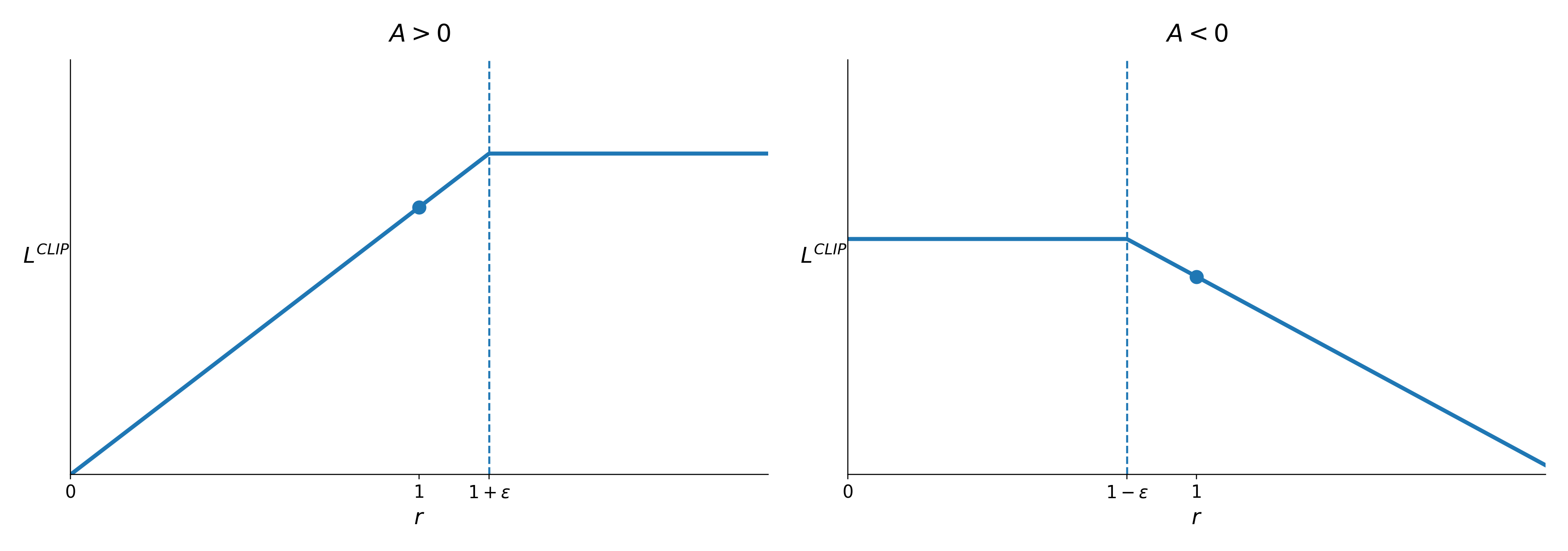
• Without a restriction, the policy may change too much in a single update.

Clipped Surrogate Objective

$$J^{CLIP}(\theta) = \hat{\mathbb E}_t \left[ \min ( \underbrace{r_t(\theta)\hat A_t}_{\text{Normal Policy Gradient objective}}, \underbrace{\operatorname{clip} (r_t(\theta),1-\epsilon,1+\epsilon)}_{\text{Clipped Policy Gradient Objective}}\hat A_t ) \right]$$

• $r_t(\theta) = \frac{\pi_\theta(a_t|s_t)}{\pi_{\theta_{\text{old}}}(a_t|s_t)}$ is the ratio of the new policy to the old policy.
• $\hat A_t = Q(s_t,a_t) - V(s_t)$ is the advantage function.
• $\epsilon$ is a hyperparameter, usually $0.1$ or $0.2$.
• If $\epsilon=0.2$, the clipping range is $[0.8,1.2]$.
• For $\hat A_t>0$, PPO removes the benefit of increasing $r_t$ above $1+\epsilon$.
• For $\hat A_t<0$, PPO removes the benefit of decreasing $r_t$ below $1-\epsilon$.
• The policy ratio itself is not strictly forced to remain inside the clipping range.
• Instead, clipping removes the incentive for excessively large beneficial policy updates.

$$\begin{array}{l} \textbf{Algorithm: PPO with Clipped Objective} \\ \textbf{Input: } \theta_0,\ \epsilon \\ \textbf{for } k=0,1,2,\ldots \textbf{ do} \\ \qquad \text{Collect set of partial trajectories } \mathcal{D}_k \text{ on policy } \pi_k=\pi(\theta_k) \\ \qquad \text{Estimate advantages } \hat{A}_t^{\pi_k} \text{ using any advantage estimation algorithm} \\ \\ \qquad \text{Compute policy update} \\ \qquad \theta_{k+1} = \arg\max_{\theta} \mathcal{L}_{\theta_k}^{CLIP}(\theta) \\ \\ \qquad \text{by taking } K \text{ steps of minibatch SGD (via Adam), where} \\ \qquad \mathcal{L}_{\theta_k}^{CLIP}(\theta) = \mathbb{E}_{\tau\sim\pi_k} \left[ \sum_{t=0}^{T} \min \left( r_t(\theta)\hat{A}_t^{\pi_k}, \operatorname{clip} \left( r_t(\theta),1-\epsilon,1+\epsilon \right) \hat{A}_t^{\pi_k} \right) \right] \\ \end{array}$$

• $\theta_0$: Initial policy parameters.
• $\epsilon$: Clipping threshold.
• $\hat{A}_t^{\pi_k}$: $A_\pi(s,a)=Q_\pi(s,a)-V_\pi(s)$, where $a_t\sim\pi(a_t\mid s_t),\quad s_{t+1}\sim P(s_{t+1}\mid s_t,a_t)$, for $t\ge0$.