RL 009
· 11 min read

Function Approximation
- Incremental methods for prediction
- Model-free VFA: MC and TD targets
GPI, Generalized Policy Iteration
- Iterate between policy evaluation and policy improvement
- Policy Evaluation: Approximate policy evaluation.
- Policy Improvement: -greedy policy improvement.
Types of Action-Value FA
- State Value Function Approximation
- Action Value Function Approximation
- The network output is a vector of Q-values for each action.
- More convenient to use discrete action spaces.
| Action | Q-value |
|---|---|
| Left | 3.2 |
| Right | 8.7 |
| Jump | 5.3 |
Action VFA
- Approximate the Action-value function.
- Doing action at state , Approximate the Q-value of that action.
- Minimize mean-squared error (MSE) between the approximate Q-value and the true Q-value .
- Use SGD to find the local minimum.
- tells us how much the prediction is off from the target.
- tells us how each weight affects the predicted -value.
Linear Action VFA
- Feature vector is used to represent the state and action pair.
- Predicted Q-value is a linear combination of the feature values. (sum of each feature value multiplied by the weight )
- : features of the state and action pair.
- : weights that need to be learned.
- derivative with respect to .
- e.g. , then
Incremental Prediction Algorithm
- Assumption so far: is given.
- But an actual RL agent does not know the true .
- Therefore, we need to estimate a target.
- Monte Carlo (MC): the target is the return .
- Update:
- It compares the predicted Q-value with the actual return observed after the episode.
- MC does not use another prediction inside the target.
- Temporal Difference (TD): the target is .
- Update:
- It compares the current Q prediction with the current reward plus the discounted next Q prediction.
- Bootstrapping: update the current prediction using another prediction.
- Because the next prediction can also be wrong, we ask: can repeated updates converge to a stable value?
- On-policy: behavior policy = target policy.
- Off-policy: behavior policy target policy.
- The policy that generates the experience is different from the policy that we want to evaluate or improve.
| Policy | Algorithm | Lookup Table | Linear | Non-linear |
|---|---|---|---|---|
| On-policy | MC | ✓ | ✓ | ✓ |
| On-policy | TD(0) | ✓ | ✓ | ✗ |
| Off-policy | MC | ✓ | ✓ | ✓ |
| Off-policy | TD(0) | ✓ | ✗ | ✗ |
- Deadly Triad: Function Approximation + Bootstrapping + Off-policy.
| Algorithm | Lookup Table | Linear | Non-linear |
|---|---|---|---|
| MC Control | ✓ | (✓) | ✕ |
| SARSA | ✓ | (✓) | ✕ |
| Q-Learning | ✓ | ✕ | ✕ |
- SARSA learns the policy that it actually follows.
- Target: , On-policy TD
- Q-Learning learns the optimal policy.
- Target: , Off-policy TD
- (✓): Moved around the near-optimal value function.
- Linear FA may not represent the exact because all state-action values share the same weight vector and must fit the same linear function.
- x: Divergence
Batch Methods
- Incremental learning: an experience -> update the weights.
- Batch methods: collect experiences -> store in -> reuse for training.
- It seeks to find the best fitting value functions.
- Which makes fit all stored data best?
- Using the agents' experience or training data.
- Training data: a fixed batch of previously collected data.
Least Squares Prediction
- Given a value function approximation:
- Given experience data: consisting of state-value pairs.
- is the sum of all squared prediction errors.
- The Least Squares method finds the parameter vector that minimizes the squared error between and .
- If we use the mean squared error instead:
- The factor does not change the minimizing .
SGD Procedure
- Sample a pair from .
- Apply the SGD update:
- Sample from -> calculate the error -> update -> repeat.
- Under appropriate conditions, SGD converges toward the Least Squares solution.
- Then, what model should represent ?
- Linear function approximator
- ANN
- CNN
DNN, Deep neural network
- Universal function approximator
- Linear FA limited to linear combinations of features
- DNN can represent non-linear mappings of features.
- Combination of both Linear and Non-Linear transformations
- It may require exponentially less nodes or parameters to represent the sample Linear function.
- SGD can be used to learn parameters
- prediction -> loss -> gradient -> SGD -> update.
- It can generalize from observed states to unseen states.
- It can handle continuous state spaces, which are common in real world problems.
- E2E learning (learn feature representation and policy together) can be more effective.
- Function approximation using images, environments with visual observations.
- DNNs can directly process pixel data and learn from raw images.
- DNNs can be used in environments with continuous action spaces for approximating policies (Robotics)
- It can achieve SOTA performance in several complex tasks.
CNN, Convolutional neural network
- CONV is the first layer to extract features from an input image.
- Core building block of a CNN
- A number of filters such as Edge Detectors are applied to the input image.
- Padding: add extra pixels around the image to handle edge cases.
- Valid Padding: no padding, output size is smaller than input size.
- .
- Output size:
- : filter size.
- Same Padding: add padding so that output size is the same as input size.
- Valid Padding: no padding, output size is smaller than input size.
- Stride: the number of pixels the filter moves across the input image.
- : Move the filter by one pixel horizontally and vertically.
- : Move the filter by two pixels horizontally and vertically.
- POOL: down sampling operation which reduces the dimensionality of a matrix.
- It reduces the number of parameters for large image but retain the valuable information.
- Max pooling:
Max(7, 8, 9, 10) = 10 - Average pooling:
Avg(7, 8, 9, 10) = 8.5 - Sum pooling:
Sum(7, 8, 9, 10) = 34
- FC: The output matrix after convolution layer is flattened and feed into a fully connected layer similar to ANN.
- It's a traditional Multi-layer Perceptron/Neural Network.
- For multi-class classification, Softmax activation function is usually used.
- Output of the CONV and POOL layers represent a high-level features of the Input image.
- FC layer uses this feature to classify the input image into the desired class.
Deep Reinforcement Learning
- Use DNNs to represent
- Value and Q-Value function (Action-value function)
- Policy (Policy Gradient methods)
- Model
- Use SGD to optimize loss function.
- RL makes the target, SGD trains DNN to fit the target.
- In TD:
- TD error:
- In Q-Learning: is the target.
Q-Learning with VFA
- Original Q-Learning converges to the optimal using look-up table.
- VFA Q-Learning minimizes MSD Loss by SGD using target Q estimates instead of true Q.
- so it can diverge due to the correlation between samples or Non-stationary targets.
Experience Replay
Environment
    │
    │ experience
    ▼
(s, a, r, s')
    │
    ▼
Replay Buffer D
┌──────────────────────┐
│ old experience       │
│ old experience       │
│ old experience       │
│ old experience       │
└──────────────────────┘
    │
    │ random sample
    ▼
Mini-batch
    │
    ├──────────────► Current Q Network
    │                   │
    │                   ▼
    │                 Q(s,a)
    │
    └──────────────► Target calculation
                        │
                        ▼
              r + γ max Q(s',a')
                        │
                        ▼
             Target − Prediction
                        │
                        ▼
                       SGD
                        │
                        ▼
                  Update weights
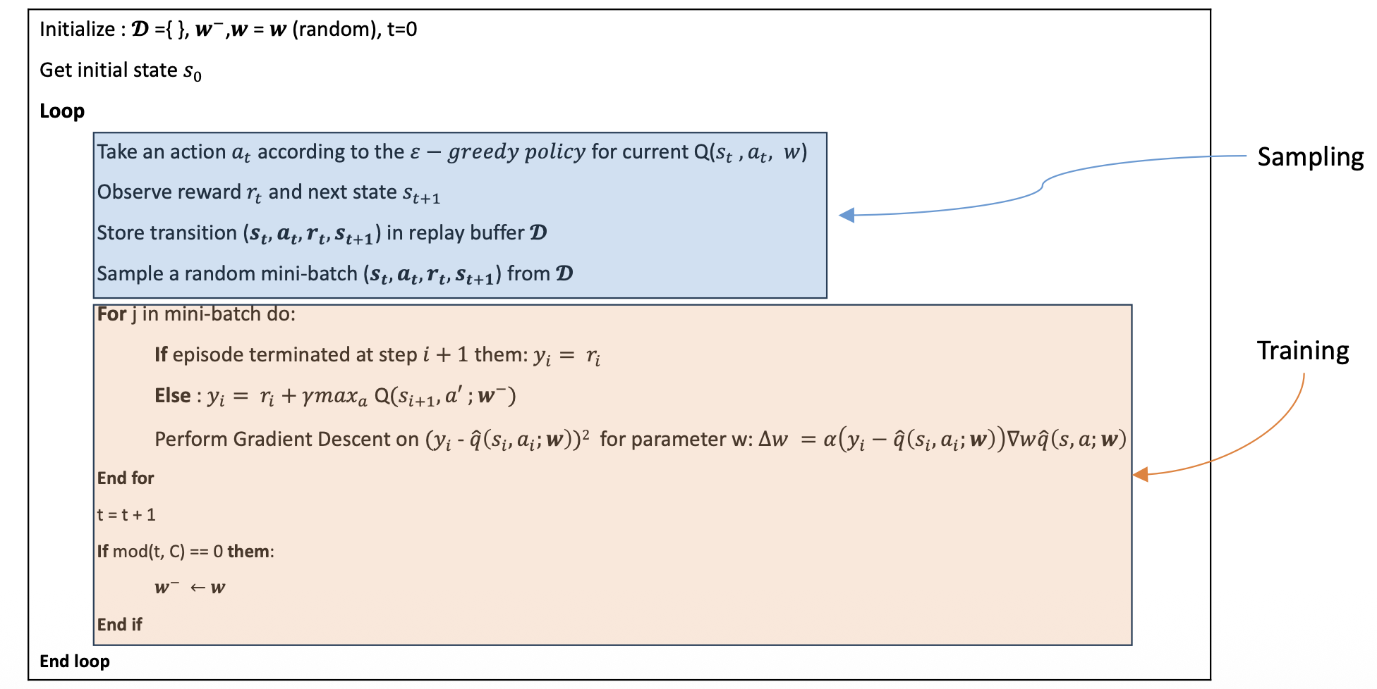
- DQN stores past transitions in a replay buffer and randomly samples them for training, which reduces correlation between consecutive samples and improves training stability.
- Sample from
- Compute the target value of the samples
- Use SGD to update the network weight:
Fixed Q-Targets
        [Same structure of network 2]

Current state s                    Next state s'
     │                                  │
     ▼                                  ▼
Online Q Network                  Target Network
weights = w                       weights = w⁻
     │                                  │
     ▼                                  ▼
Q(s,a;w)                      max Q(s',a';w⁻)
     │                                  │
     └────────── compare ────────────────┘
                      │
                      ▼
                    Loss
                      │
                      ▼
                update only w
- Improve stability by fixing the target weights used in the target calculation for multiple updates.
- Target network uses different set of weights that the weights being updated.
- : set of weights used in the target.
- : set of weights being updated.
- Sample from
- Compute the target value of the samples
- Use SGD to update the network weight:
DQN
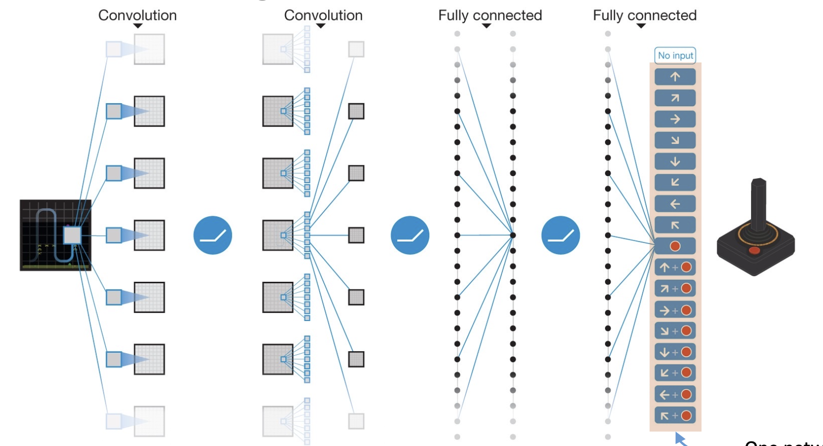
DQN in Atari
- E2E learning of s$
- Input state is a stack or raw pixels from last 4 frames.
- Output is for 18 joystick/button positions
- Reward is chance in score for that step.
- Network Architecture and hyper-parameters are fixed across all games.
- 4x84x84 stack of 4 previous frames -> 16 8x8 filters CONV -> 32 4x4 filters CONV -> 256 hidden units FC -> Fully connected linear output layer.