IPPR 003

Feature Detection

1. Detect invariant features of the image.
2. Describe the local area around each feature.
3. Match patterns of the feature descriptions.

Moravec conner detector

$E(u, v) = \sum_{x, y} [I(x, y) - I(x + u, y + v)]^2$

• One of the earliest corner detectors (1980)
• Moravec detects a corner by shifting a small window in different directions and checking whether the image changes significantly in every direction.
  • Shifting a window in any direction should give a large change in intensity, measured in terms of Sum of Squared Differences (SSD).
• $(u, v)$ is how much the window is shifted.
• Larger $E$ indicates the image changes more after the shift.

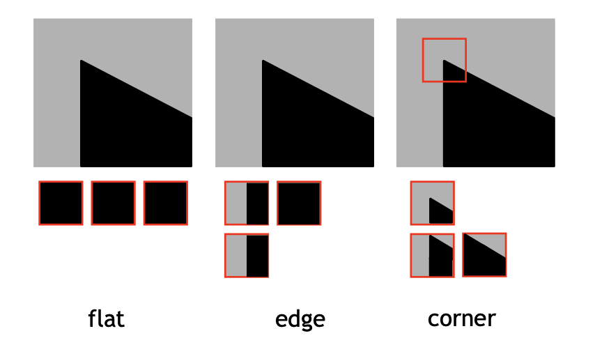
• Flat: $E \approx 0$, No change in any direction
• Edge: $E \approx 1$, Change in some direction
• Corner: $E \approx 40$, Large change in every direction

Harris corner detector

$E(x, y) = \sum_{u}\sum_{v} \underbrace{W(u, v)}_{\text{Window function}} [\underbrace{I(u + x, v + y)}_{\text{Shifted Intensity}} - \underbrace{I(u, v)}_{\text{Intensity}}]^2$

• Improvement over Moravec change of intensify for a shifted windoe centered at $(u, v)$

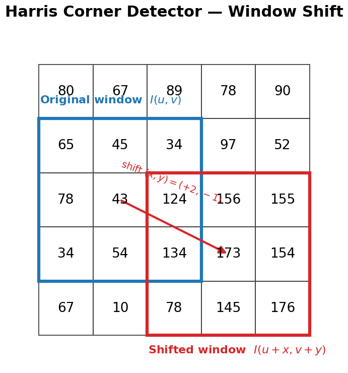
• $(x, y) = (1, 0) \rightarrow$ move 1px to the right.
• $(x, y) = (0, 1) \rightarrow$ move down 1px.
• $(x, y) = (2, 1) \rightarrow$ move 2px to the right and 1px down.
• $I(u, v)$: Pixel intensity of the original point.
• $I(u + x, v + y)$: Pixel intensity of the shifted point.
• SSD: if $I(u,v) = 65$, and $I(u + x, v+ y) = 124$, then the SSD is $(124 - 65)^2 = 3481$.
• $w(u, v)$: window function, usually apply gaussian weighting to the pixels around the center.
  • if we calculate all the $(x, y)$ step by step, it will be computationally expensive.
  • so we use Taylor Expansion to approximate the intensity change.

Taylor Expansion

$I(u + x, v + y) \approx I(u, v) + I_x(u, v)x + I_y(u, v)y$

• Let $I_x$ and $I_y$ be the partial derivatives of $I$
• Approximates the intensity of the slightly shifted point, using the current intensity and gradient information.
• $I_x = \frac{\partial I}{\partial x}$: How much the intensity changes when moving to the right or left a little bit.
• $I_y = \frac{\partial I}{\partial y}$: How much the intensity changes when moving up or down a little bit.

$E(x, y) \approx \sum_{u}\sum_{v} w(u, v) [I_x(u, v)x + I_y(u, v)y]^2$

• because $I(u + x, v + y) \approx I(u, v) + I_x(u, v)x + I_y(u, v)y$.
• we can calculate intensity change by x/y gradient and the window shift.
• $(ax + by)^2 = a^2x^2 + 2abxy + b^2y^2 = [x, y] \begin{bmatrix} a^2 & ab \\ ab & b^2 \end{bmatrix} \begin{bmatrix} x \\ y \end{bmatrix}$

$E(x,y) = [x, y] \underbrace{\begin{bmatrix} \sum_{u}\sum_{v} w(u, v) I_x^2 & \sum_{u}\sum_{v} w(u, v) I_xI_y \\ \sum_{u}\sum_{v} w(u, v) I_xI_y & \sum_{u}\sum_{v} w(u, v) I_y^2 \end{bmatrix}}_{A} \begin{bmatrix} x \\ y \end{bmatrix}$

• Eigenvector = direction of the change
• Eigenvalue = magnitude of the change
• if both $\lambda_1 \text{ and } \lambda_2 \approx 0$, the point is flat.
• if either $\lambda_1 \text{ or } \lambda_2 \gg 0$ the point is an edge.
• if both $\lambda_1 \text{ and } \lambda_2 \ll 0$ the point is a corner.

$R = \det(A) - k(\text{trace}(A))^2$

• $\det(A) = \lambda_1 \lambda_2$
  • it can check if the point is a corner by checking if $\lambda_1 \text{ and } \lambda_2$ are both large.
• $\text{trace}(A) = \lambda_1 + \lambda_2$
  • it can penalizes edge-like responses where one eigenvalue is large but the other is small.
• $R = \lambda_1 \lambda_2 - k(\lambda_1 + \lambda_2)^2$
  • $k$ is an empirical constant, typically set $0.04 \leq k \leq 0.06$.
  • A threshold is applied an corners detected, non-maxima are suppressed.
  • $R$ can be derived from eigenvalues of the matrix $A$.
  • $R \approx 0$ the point is flat.
  • $R < 0$ the point is an edge.
  • $R \gg 0$ the point is a corner.

Harris corner detection pipeline

• Compute the Harris response $R$ for every pixel.
• Large positive $R$ indicates a strong corner response.
• Apply a threshold to remove weak responses.
• Apply non-maximum suppression to keep only local maxima.
• Overlay the remaining points on the original image as detected corners.

Detector vs descriptor

• Detector: detect the location of the features in an image or video (WHERE).
• Descriptor: descriptors summarize the appearance of the neighborhood (WHAT IT LOOKS LIKE).
• A good feature detector should be:
  • make similar descriptors for similar features of the same object.
  • Invariance: the descriptor should be invariant to translation, rotation, scale, and illumination.

SIFT

Scale-Invariant Feature Transform

• It was proposed by Lowe in 1999, includes both a detector and a descriptor.
• A method to detect and match local features despite changes in scale and rotation.
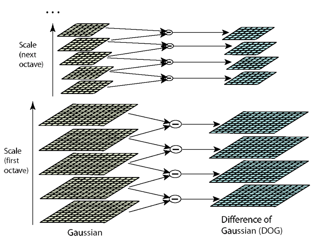
• Core idea: build multiple blurred versions of the image, compute their differences, and find points that stand out across scales.

1. Build a scale-space pyramid of Differences of Gaussians (DoG) and detect minima/maxima.
2. Localize keypoints.
3. Assign them an orientation.
4. Compute the SIFT descriptor.

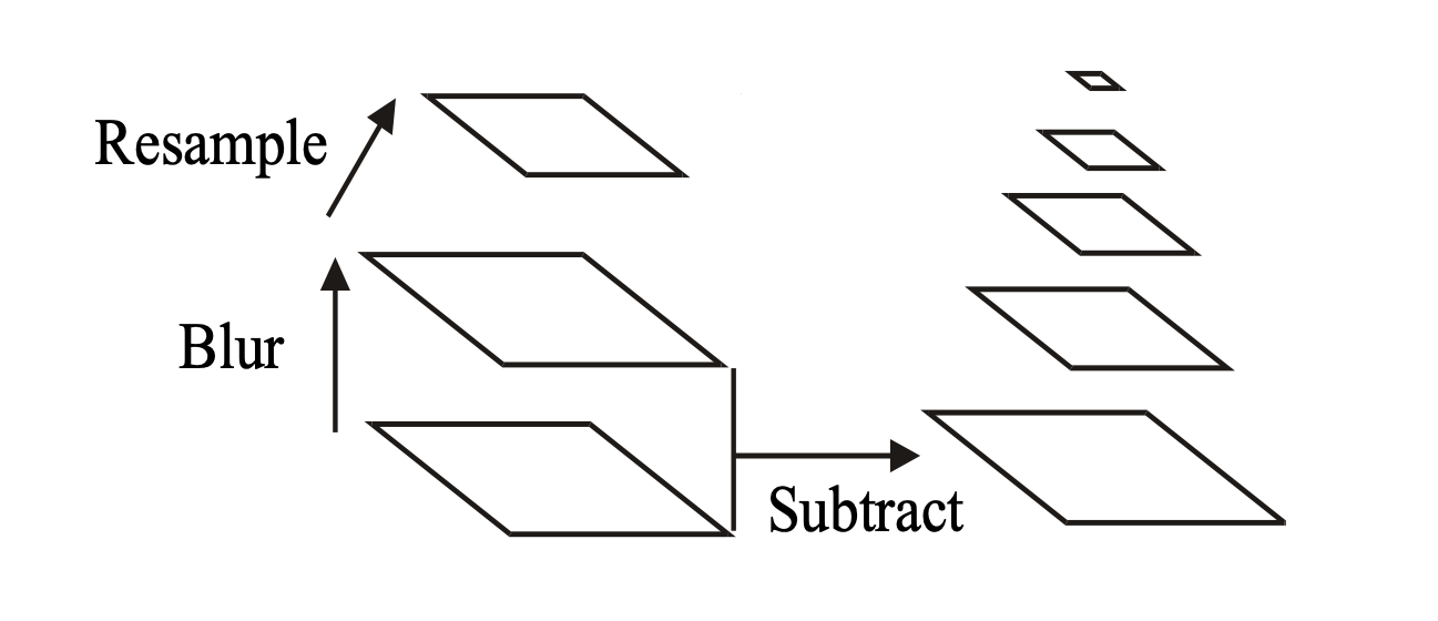
• $L(x, y, \sigma) = G(x, y, \sigma) * I(x, y)$: Blurred image at scale $\sigma$.
• $D(x, y, \sigma) = L(x, y, k\sigma) - L(x, y, \sigma)$: Difference of Gaussians at scale $\sigma$.
• Octave: a group of scale-space images at the same resolution.
• After each octave, the image is typically downsampled by a factor of 2.

Key point localization

$\text{Image} \rightarrow \text{Gaussian scale space} \rightarrow \text{DoG} \rightarrow \text{DoG extrema} \rightarrow \text{Filter low-contrast and edge responses} \rightarrow \text{Keypoints}$

• Detect local maxima and minima in DoG scale space.
• Remove low-contrast points because they are unstable and sensitive to noise.
• Remove edge responses because their locations are poorly localized.
• Use the ratio of principal curvatures to distinguish edges from stable corner/blob-like features.
• Example: $832 \rightarrow 729 \rightarrow 536$

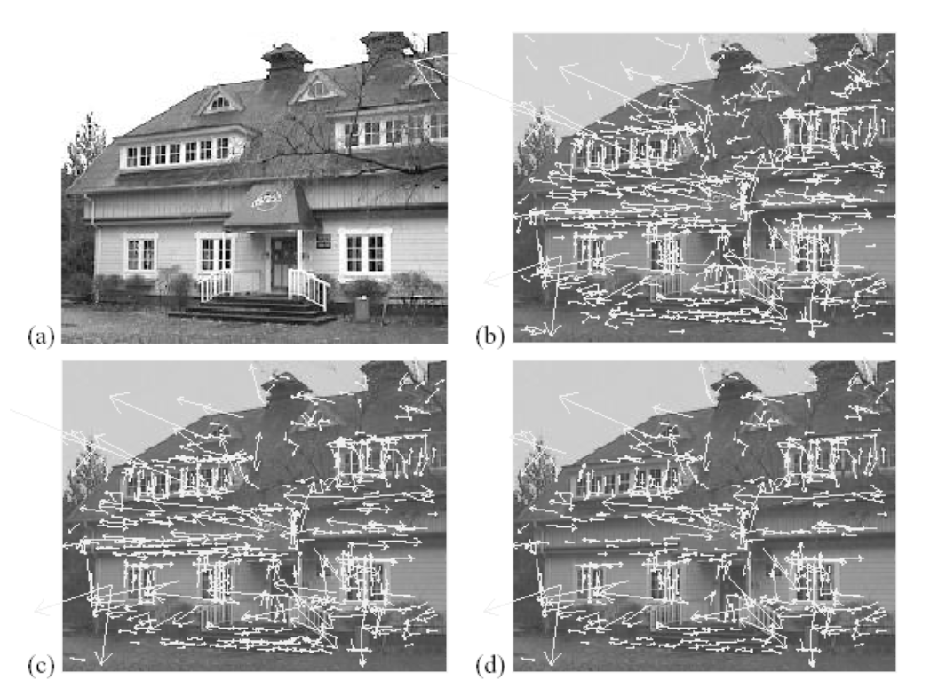
• (a): Original image (233x189)
• (b): 832 DoG extrema
• (c): 729 left after peak-value threshold
• (d): left after testing the ratio of principal curvatures.

Orientation assignment

• For every keypoint, compute the gradient at each location in its local neighborhood.
• The gradients are computed on the Gaussian-blurred image at the keypoint's scale, $\sigma$.
• Gradient directions are quantized into 36 bins over $360^\circ$.
• Each gradient contributes to the histogram according to its magnitude.
• The dominant histogram bin is assigned as the keypoint's orientation.
  • $[10, 20, 20, 30, 20] \rightarrow 20$
  • This orientation becomes the anchor direction for the SIFT descriptor.

SIFT descriptor

SIFT descriptor = 128-dimensional vector

• A 16x16 grid of locations of the gradient at $\sigma$ scale around the keypoint.
• The grid is divided into 4x4 sub-grids of 4x4 locations each.
• For each sub-grid, an 8-bin histogram of the magnitude weighted gradient orientation is computed.
  • All 8 bins are retained.
• The histogram from all the sub-grids are concatenated into the SIFT descriptor.
  • The dimensionality is given by 8 bins x 16 histograms = 128.

$\text{Image} \rightarrow \text{Gaussian scale space} \rightarrow \text{DoG} \rightarrow \text{DoG extrema} \rightarrow \text{Filter low-contrast and edge responses} \rightarrow \text{Keypoints} \rightarrow \text{Assign orientation} \rightarrow \text{Build 128-D descriptor}$

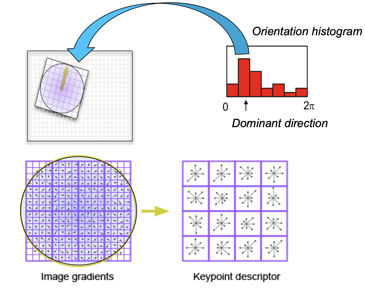
• SIFT Features encode information about at 16x16 area around the feature point at the appropriate scale.
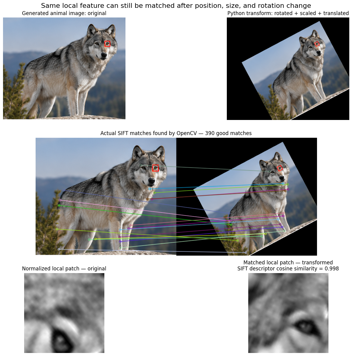
• It is scale, rotation, and translation invariant.
• Similar features give similar SIFT values regardless of orientation, scale, and translation.

Applications of SIFT

• Object recognition: SIFT descriptors are extracted from an input image and matched to the SIFT descriptors of known objects in a database.
• Stereo vision: SIFT descriptors from the left and right images are matched to create the disparity map.
• Tracking: SIFT descriptors from successive frames are matched to track a target.
• Object and action classification: histograms of SIFT descriptors are computed over single frames or whole videos and used as input for a classifier.

Object classification

• Object classification uses histograms of SIFT descriptors to characterize the class of an object.
• A popular histogram representation is called Bag of Features (BoF).
  • BoF first requires creating a dictionary, also called a codebook, from the training set.
  • Once the dictionary is computed, a Bag of Features can be computed for any image.
  • The resulting Bag of Features is then used for classification.

# Example SIFT descriptors from training images
descriptors = [
    [1.0, 1.2],
    [0.9, 1.1],
    [1.1, 0.8],

    [5.0, 5.1],
    [4.8, 5.2],
    [5.2, 4.9],

    [9.0, 1.0],
    [8.8, 1.2],
]

# Representative descriptors after clustering
codebook = [
    [1.0, 1.0],   # codeword 1
    [5.0, 5.0],   # codeword 2
    [9.0, 1.0],   # codeword 3
]

# SIFT descriptors from a new image
new_image_descriptors = [
    [1.2, 0.9],
    [0.8, 1.1],
    [5.1, 4.9],
    [9.2, 1.1],
    [8.9, 0.8],
]

# Nearest codeword assignments
assignments = [
    0,  # -> codeword 1
    0,  # -> codeword 1
    1,  # -> codeword 2
    2,  # -> codeword 3
    2,  # -> codeword 3
]

# Bag of Features histogram
bof = [2, 1, 2]

Dictionary creation

• Extract all SIFT descriptors from the training images.
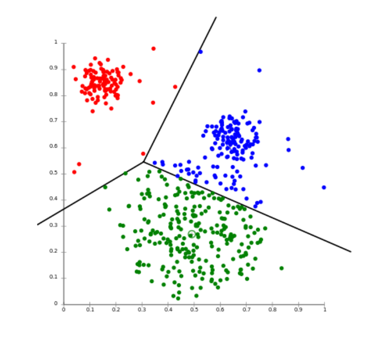
• Use a clustering algorithm, typically k-means, to group the descriptors into $k$ clusters.
• The descriptor space is partitioned into $k$ regions.
  • Example: $k=1000$.
• The resulting clusters form the dictionary/codebook.

Bag of Features

• Map all SIFT descriptors of an image to clusters in the dictionary.
• Count the number of descriptors assigned to each cluster.
• Form a histogram with $k$ bins.
• Use this histogram as a measurement vector for a classifier.
• Possible classifiers include Bayes, SVM, KNN, and neural networks.

Other Local Features

• SURF (Speeded Up Robust Features): another local feature method designed to provide robust features with faster computation.
• GLOH (Gradient Location and Orientation Histogram): describes local image structure using gradient location and orientation histograms.
• HOG (Histogram of Oriented Gradients): represents local regions using histograms of gradient orientations.
• For classification, descriptors can be extracted either from detected interest points or from a regular grid.
• Descriptors extracted from a regular grid are called dense features.

Spatio-temporal local features

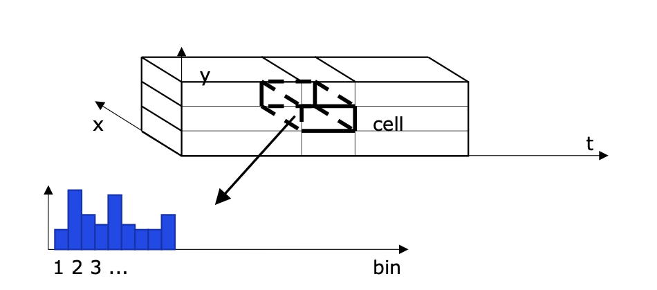
• In video, local features can be extracted from each frame separately or as 3D local features.
• Here, “3D” means $x, y, t$, where $t$ is time.
• These are called spatio-temporal features.
• They describe the appearance of local cuboids across space and time.

Other Spatio-temporal local features

• HOG/HOF: Histogram of Optical Flow.
• HOG3D: a spatio-temporal extension of HOG.
• ESURF: Extended SURF.
• MBH: Motion Boundary Histograms.
• DTF: Dense Trajectory Features.
• For classification, these descriptors can be computed either at detected points or over a regular grid.

Object Classification FLow

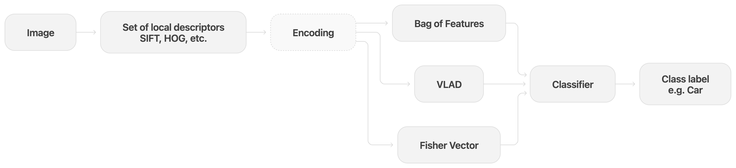
• Local descriptors: An image is represented by many local feature descriptors such as SIFT or HOG. The result is a set of descriptors, not a single vector.
• Encoding: Since different images can produce different numbers of descriptors, the set of descriptors is converted into one fixed-length vector. Bag of Features, VLAD, and Fisher Vector are different encoding methods for this purpose.
  • Bag of Features: Each descriptor is assigned to the nearest representative feature, and the number of descriptors assigned to each representative feature is counted.
  • VLAD: Instead of only counting assignments, VLAD stores how each descriptor differs from its nearest representative feature.
  • Fisher Vector: It represents how the descriptors differ from a learned feature distribution, capturing more detailed statistical information.
• Classifier: The encoded fixed-length vector is given to a classifier, which outputs a class label such as car, person, or dog.
• Main idea: SIFT describes many local regions, while BoF, VLAD, and Fisher Vector combine those local descriptions into one image-level vector for classification.