RL 004

· 16 min read

Bellman Equation​

vπ(s)=Eπ[Rt+1⏟Immediate Reward+γvπ(St+1)⏟Discounted Future Value  |  St=s⏟Starting at state s]v_\pi(s) = \mathbb{E}_\pi \left[ \underbrace{R_{t+1}}_{\text{Immediate Reward}} + \gamma \underbrace{v_\pi(S_{t+1})}_{\text{Discounted Future Value}} \;\middle|\; \underbrace{S_t = s}_{\text{Starting at state s}} \right]

  • Fundamental concept in RL using a recursive equation to express a way to compute the value of a state based on the values of its successor states.
v(s)=E[Rt+1+γRt+2+γ2Rt+3+…  |  St=s]=E[Rt+1+γ(Rt+2+γRt+3+… )⏟Gt+1  |  St=s]=E[Rt+1+γGt+1  |  St=s]=E[Rt+1+γv(St+1)  |  St=s]=E[Rt+1∣St=s]⏟Immediate Reward R(s)+γ E[v(St+1)∣St=s]⏟Expected Next State Value(∵E[X+γY]=E[X]+γE[Y])=R(s)+γ∑s′P(s′∣s)v(s′)⏟Transition Dynamics(∵E[g(X)]=∑xP(x)g(x))\begin{aligned} v(s) &= \mathbb{E} \left[ R_{t+1} + \gamma R_{t+2} + \gamma^2 R_{t+3} + \dots \;\middle|\; S_t = s \right] \\[8pt] &= \mathbb{E} \left[ R_{t+1} + \gamma \underbrace{\left( R_{t+2} + \gamma R_{t+3} + \dots \right)}_{G_{t+1}} \;\middle|\; S_t = s \right] \\[8pt] &= \mathbb{E} \left[ R_{t+1} + \gamma G_{t+1} \;\middle|\; S_t = s \right] \\[8pt] &= \mathbb{E} \left[ R_{t+1} + \gamma v(S_{t+1}) \;\middle|\; S_t = s \right] \\[8pt] &= \underbrace{\mathbb{E}[R_{t+1} \mid S_t = s]}_{\text{Immediate Reward } \mathcal{R}(s)} + \gamma \, \underbrace{\mathbb{E}[v(S_{t+1}) \mid S_t = s]}_{\text{Expected Next State Value}} && (\because \mathbb{E}[X + \gamma Y] = \mathbb{E}[X] + \gamma\mathbb{E}[Y]) \\[10pt] &= \mathcal{R}(s) + \gamma \underbrace{\sum_{s'} \mathcal{P}(s' \mid s) v(s')}_{\text{Transition Dynamics}} && \left(\because \mathbb{E}[g(X)] = \sum_x P(x)g(x)\right) \end{aligned}

Bellman Equation Example​

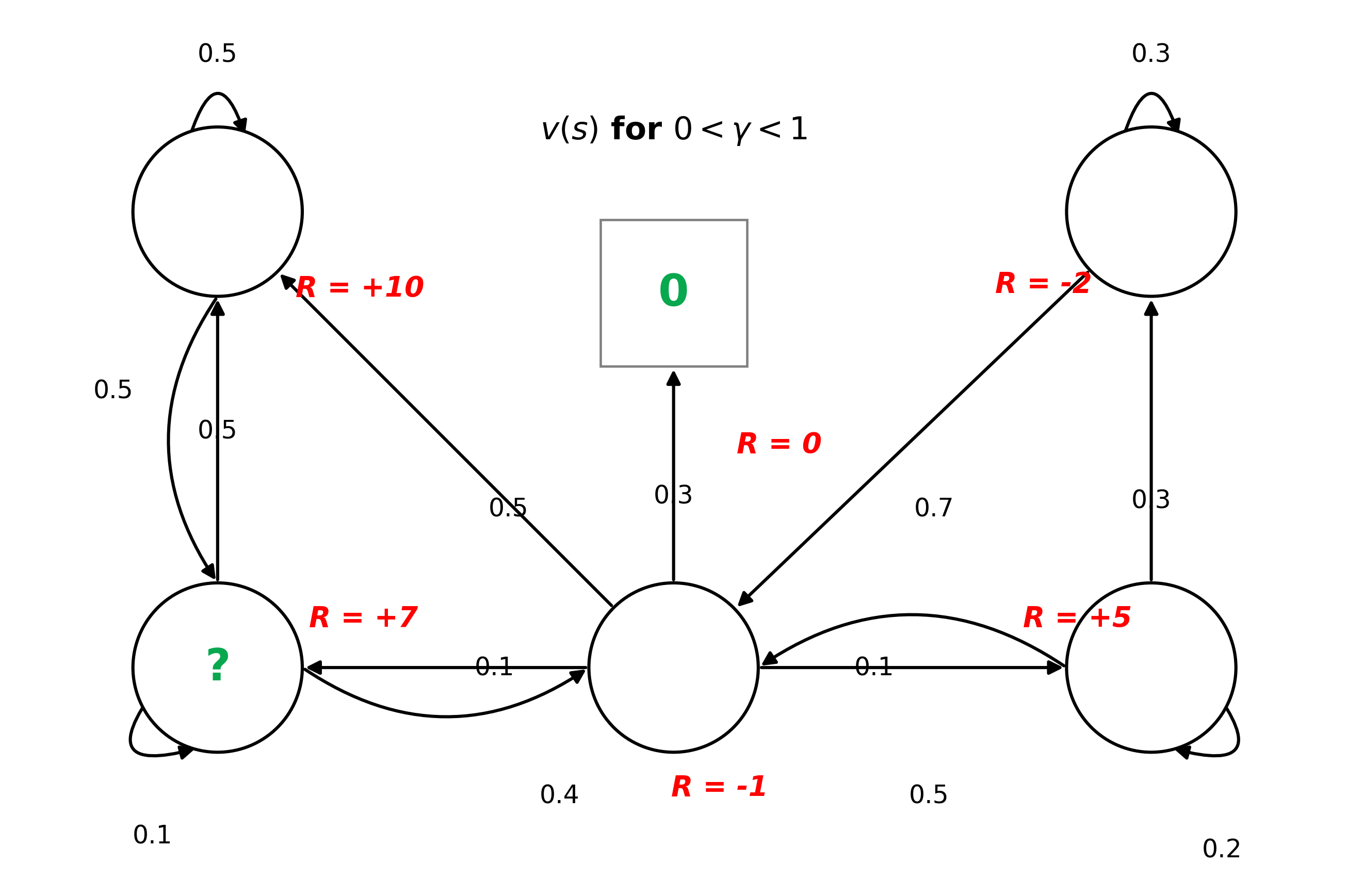
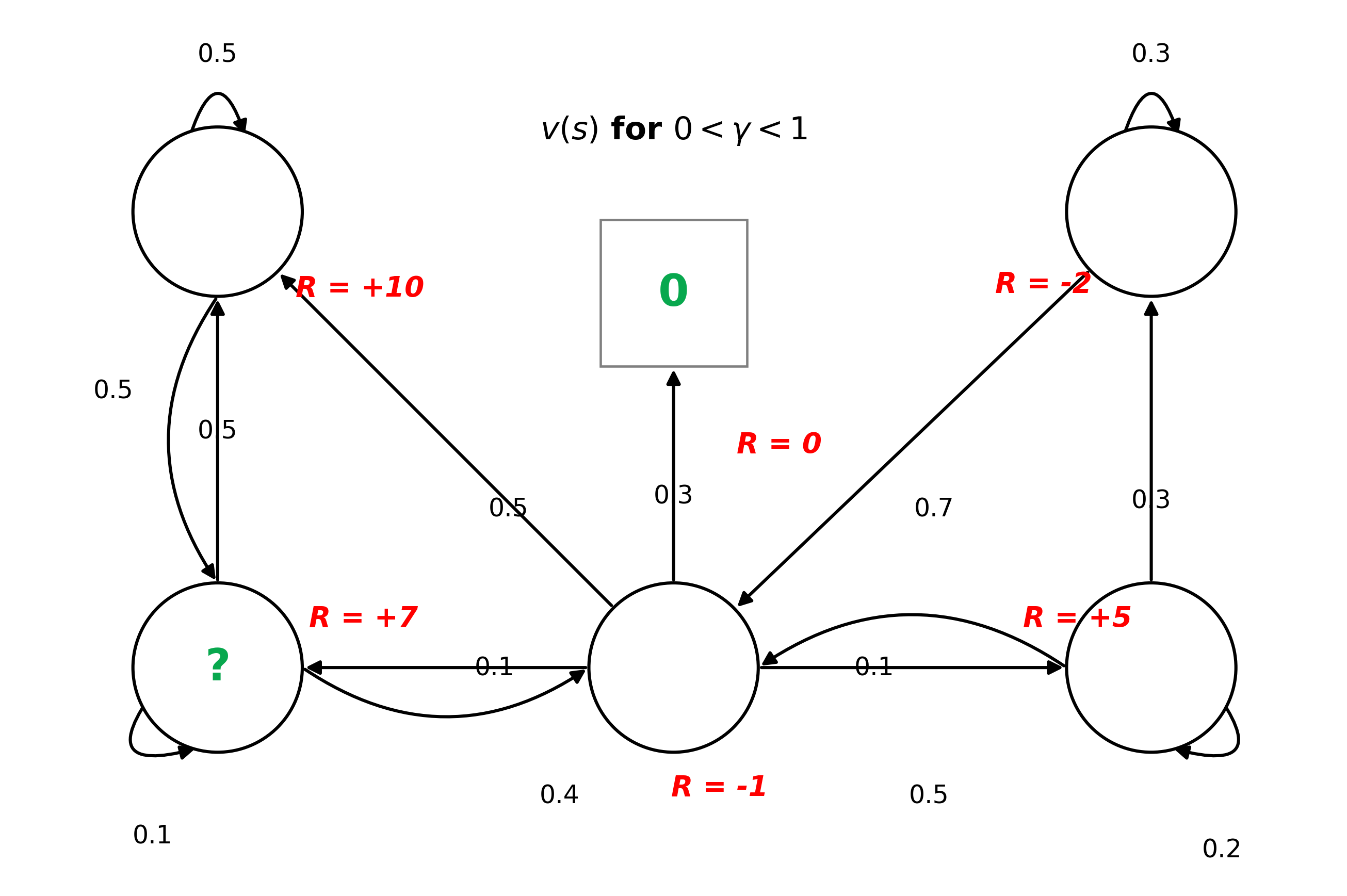
Bellman Example

v(sBL)=7+γ(0.1⋅v(sBL)+0.5⋅(sTL)+0.4⋅(sBR))v(s_{\text{BL}}) = 7 + \gamma(0.1 \cdot v(s_{\text{BL}}) + 0.5 \cdot(s_{TL}) + 0.4 \cdot(s_{BR}))

Bellman Equation in Matrix Form​

v=R+γPvv = \mathcal{R} + \gamma \mathcal{P} v

[v(s1)⋮v(sn)]⏟V of a particular state=[R(s1)⋮R(sn)]⏟Immediate Reward+γ[P11⋯P1n⋮⋱⋮Pn1⋯Pnn]⏟Transition Matrix[v(s1)⋮v(sn)]⏟V of future state\begin{aligned} \underbrace{ \begin{bmatrix} v(s_1) \\ \vdots \\ v(s_n) \end{bmatrix}}_{\text{V of a particular state}} = \underbrace{\begin{bmatrix} \mathcal{R}(s_1) \\ \vdots \\ \mathcal{R}(s_n) \end{bmatrix}}_{\text{Immediate Reward}} + \gamma \underbrace{\begin{bmatrix} \mathcal{P}_{11} & \cdots & \mathcal{P}_{1n} \\ \vdots & \ddots & \vdots \\ \mathcal{P}_{n1} & \cdots & \mathcal{P}_{nn} \end{bmatrix}}_{\text{Transition Matrix}} \underbrace{\begin{bmatrix} v(s_1) \\ \vdots \\ v(s_n) \end{bmatrix}}_{\text{V of future state}} \end{aligned}

Solving the Bellman Equation​

Linear System of Equations​

v=R+γPvv−γPv=R(I−γP)v=Rv=(I−γP)−1R\begin{aligned} \mathcal{v} &= \mathcal{R} + \gamma \mathcal{P}\mathcal{v} \\ \mathcal{v} - \gamma \mathcal{P}\mathcal{v} &= \mathcal{R} \\ (I - \gamma \mathcal{P})\mathcal{v} &= \mathcal{R} \\ \mathcal{v} &= (I - \gamma \mathcal{P})^{-1} \mathcal{R} \end{aligned}
  • Computational Complexity: O(n3)O(n^3)
  • For small MDPs: direct solution is possible (up to 100 states)
  • For large MDPs:
    • Iterative methods
    • Dynamic Programming
    • Monte Carlo Tree
    • TD learning

State-Value Function​

vπ(s)⏟Value of state s=Eπ⏟Follows policy π[Rt+1⏟Immediate Reward+γvπ(St+1)⏟Discounted Value of Next State  |  St=s⏟Starting at state s]\begin{aligned} \underbrace{v_\pi(s)}_{\text{Value of state } s} = \underbrace{\mathbb{E}_\pi}_{\text{Follows policy } \pi} \left[ \underbrace{R_{t+1}}_{\text{Immediate Reward}} + \gamma \underbrace{v_\pi(S_{t+1})}_{\text{Discounted Value of Next State}} \;\middle|\; \underbrace{S_t = s}_{\text{Starting at state } s} \right] \end{aligned}
  • Evaluates the expected return starting from state ss and following policy π\pi thereafter.
  • How good is it to be in state ss?
  • vπ(s)v_\pi(s): Expected cumulative return starting from state ss under policy π\pi.
  • Eπ\mathbb{E}_\pi: Expectation over action selections (At∼πA_t \sim \pi) and transition dynamics (St+1∼PS_{t+1} \sim \mathcal{P}).
  • Rt+1R_{t+1}: Immediate reward received upon transitioning out of state ss.
  • γvπ(St+1)\gamma v_\pi(S_{t+1}): Discounted expected value of the next successor state St+1S_{t+1}.
  • St=sS_t = s: Condition that the agent starts at state ss at time step tt.

vπ(s)=∑a∈Aπ(a∣s)qπ(s,a)v_{\pi}(s) = \sum_{a \in \mathcal{A}} \pi(a \mid s) q_{\pi}(s, a)

  • The value of state ss is the policy-weighted average of the values of all possible actions that can be taken from that state.
  • vπ(s)v_{\pi}(s): Expected cumulative return starting from state ss under policy π\pi.
  • π(a∣s)\pi(a \mid s): Probability of taking action aa in state ss under policy π\pi.
  • qπ(s,a)q_{\pi}(s, a): Value of taking action aa in state ss under policy π\pi.

Action-Value Function​

qπ(s,a)⏟Action-Value of (s,a)=Eπ⏟Follows policy π[Rt+1⏟Immediate Reward+γqπ(St+1,At+1)⏟Discounted Next Action-Value  |  St=s,At=a⏟Starting at s taking action a]\begin{aligned} \underbrace{q_\pi(s, a)}_{\text{Action-Value of } (s, a)} = \underbrace{\mathbb{E}_\pi}_{\text{Follows policy } \pi} \left[ \underbrace{R_{t+1}}_{\text{Immediate Reward}} + \gamma \underbrace{q_\pi(S_{t+1}, A_{t+1})}_{\text{Discounted Next Action-Value}} \;\middle|\; \underbrace{S_t = s, A_t = a}_{\text{Starting at } s \text{ taking action } a} \right] \end{aligned}
  • Evaluates the expected return of taking an arbitrary action aa in state ss, and subsequently following policy π\pi from step t+1t+1 onward.
  • How good is it to take action aa in state ss?
  • qπ(s,a)q_\pi(s, a): Value of taking action aa in state ss under policy π\pi (Q-value).
  • Eπ\mathbb{E}_\pi: Expectation over the next transition (St+1∼PS_{t+1} \sim \mathcal{P}) and the subsequent action (At+1∼πA_{t+1} \sim \pi).
  • Rt+1R_{t+1}: Immediate reward resulting from the state-action pair (s,a)(s, a).
  • γqπ(St+1,At+1)\gamma q_\pi(S_{t+1}, A_{t+1}): Discounted expected value of the successor state-action pair (St+1,At+1)(S_{t+1}, A_{t+1}).
  • St=s,At=aS_t = s, A_t = a: Condition that both the initial state and the initial action are fixed at time tt.
vπ(s)=∑a∈Aπ(a∣s)(Rsa+γ∑s′∈SPss′avπ(s′))\begin{aligned} v_\pi(s) = \sum_{a \in \mathcal{A}} \pi(a \mid s) \left( \mathcal{R}_s^a + \gamma \sum_{s' \in \mathcal{S}} \mathcal{P}_{ss'}^a v_\pi(s') \right) \end{aligned}
  • Evaluates state ss directly by averaging over all possible action branches (π\pi) and their subsequent environmental transitions (P\mathcal{P}).
  • Rsa\mathcal{R}_s^a: Immediate reward resulting from the state-action pair (s,a)(s, a).
  • γ∑s′∈SPss′avπ(s′)\gamma \sum_{s' \in \mathcal{S}} \mathcal{P}_{ss'}^a v_\pi(s'): Discounted expected value of the successor state s′s' resulting from the state-action pair (s,a)(s, a).
  • Pss′a\mathcal{P}_{ss'}^a: Probability of transitioning from state ss to state s′s' when action aa is taken.
  • S\mathcal{S}: Set of all possible states.
  • A\mathcal{A}: Set of all possible actions.
  • π(a∣s)\pi(a \mid s): Probability of taking action aa in state ss under policy π\pi.
  • vπ(s′)v_\pi(s'): Value of state s′s' under policy π\pi.

Bellman Expectation Equation​

qπ(s,a)=Rsa+γ∑s′∈SPss′a∑a′∈Aπ(a′∣s′)qπ(s′,a′)\begin{aligned} q_\pi(s, a) = \mathcal{R}_s^a + \gamma \sum_{s' \in \mathcal{S}} \mathcal{P}_{ss'}^a \sum_{a' \in \mathcal{A}} \pi(a' \mid s') q_\pi(s', a') \end{aligned}
  • Evaluates the state-action pair (s,a)(s, a) by summing immediate reward and the expected value of future action pairs (s′,a′)(s', a'), averaged across transition dynamics P\mathcal{P} and next-step policy choices π\pi.
  • Rsa\mathcal{R}_s^a: Immediate reward resulting from the state-action pair (s,a)(s, a).
  • γ∑s′∈SPss′a∑a′∈Aπ(a′∣s′)qπ(s′,a′)\gamma \sum_{s' \in \mathcal{S}} \mathcal{P}_{ss'}^a \sum_{a' \in \mathcal{A}} \pi(a' \mid s') q_\pi(s', a'): Discounted expected value of the successor state-action pair (s′,a′)(s', a') resulting from the state-action pair (s,a)(s, a).
  • Pss′a\mathcal{P}_{ss'}^a: Probability of transitioning from state ss to state s′s' when action aa is taken.
  • S\mathcal{S}: Set of all possible states.
  • A\mathcal{A}: Set of all possible actions.
  • π(a′∣s′)\pi(a' \mid s'): Probability of taking action a′a' in state s′s' under policy π\pi.
vπ(s)→Action Policy πqπ(s,a)↑↓Environment Transition Pvπ(s′)←Environment Transition Pqπ(s′,a′)\begin{matrix} v_\pi(s) & \xrightarrow{\text{Action Policy } \pi} & q_\pi(s, a) \\ \uparrow & & \downarrow \text{Environment Transition } \mathcal{P} \\ v_\pi(s') & \xleftarrow{\text{Environment Transition } \mathcal{P}} & q_\pi(s', a') \end{matrix}

Optimal Value Function​

V∗(s)=max⁡πvπ(s)V_*(s) = \max_\pi v_\pi(s)

  • The optimal State-Value Function V∗(s)V_*(s)
  • Maximum value function over all policies, or maximum possible reward that can be achieved from state ss.

q∗(s,a)=max⁡πqπ(s,a)q_*(s, a) = \max_\pi q_\pi(s, a)

  • The Optimal Action-Value Function q∗(s,a)q_*(s, a)
  • Maximum action-value function over all policies, or given state ss and action taken aa, what is the maximum reward that can be achieved from there onwards.

Optimal Policy​

π∗≥π  ⟺  vπ∗(s)≥vπ(s)∀s∈S\pi_* \geq \pi \iff v_{\pi_*(s)} \geq v_\pi(s) \quad \forall s \in \mathcal{S}

  • If certain policy is better than another policy, then the value of the better policy is greater than or equal to the value of others in all states.

Theorem fo any MDP​

  • Existence of an Optimal Policy: There always exists at least one optimal policy π∗\pi_* that is better than or equal to all other policies across all states (π∗≥π,  ∀π\pi_* \ge \pi, \; \forall \pi).
  • Uniqueness of the Optimal State-Value Function: Although multiple distinct optimal policies may exist (e.g., when two different paths yield the exact same maximum expected return), all optimal policies achieve the exact same unique optimal state-value function (vπ∗(s)=v∗(s)v_{\pi_*}(s) = v_*(s)).
  • Uniqueness of the Optimal Action-Value Function: Similarly, all optimal policies achieve the exact same unique optimal action-value function (qπ∗(s,a)=q∗(s,a)q_{\pi_*}(s, a) = q_*(s, a)).

Finding an Optimal Policy​

π∗(a∣s)={1if a=arg⁡max⁡a∈Aq∗(s,a)0otherwise\pi_*(a \mid s) = \begin{cases} 1 & \text{if } a = \arg\max_{a \in \mathcal{A}} q_*(s, a) \\ 0 & \text{otherwise} \end{cases}
  • If q∗(s,a)q_*(s, a) is known, optimal policy is achieved.
  • A deterministic optimal policy always exists for any MDP.

Bellman Optimality Equation​

Bellman Optimality Equation for v∗v_*​

v∗(s)⏟Optimal Value of State s=max⁡a∈Aq∗(s,a)⏟Optimal Value of Action a\begin{aligned} \underbrace{v_*(s)}_{\text{Optimal Value of State } s} = \max_{a \in \mathcal{A}} \underbrace{q_*(s, a)}_{\text{Optimal Value of Action } a} \end{aligned}
  • State-Value to Action-Value (s→as \rightarrow a)
  • The optimal state-value is achieved by greedily picking the single action that yields the maximum optimal action-value.
q∗(s,a)⏟Optimal Action-Value=Rsa⏟Immediate Reward+γ∑s′∈SPss′av∗(s′)⏟Expected Optimal Future Value\begin{aligned} \underbrace{q_*(s, a)}_{\text{Optimal Action-Value}} = \underbrace{\mathcal{R}_s^a}_{\text{Immediate Reward}} + \gamma \underbrace{\sum_{s' \in \mathcal{S}} \mathcal{P}_{ss'}^a v_*(s')}_{\text{Expected Optimal Future Value}} \end{aligned}
  • Action-Value to Next State-Value (a→s′a \rightarrow s')
  • Once the action aa is committed, the outcome is governed by the environment dynamics Pss′a\mathcal{P}_{ss'}^a, requiring an expectation (average) over possible successor states s′s'.
v∗(s)⏟Optimal Value of State s=max⁡a∈A(Rsa⏟Immediate Reward+γ∑s′∈SPss′av∗(s′)⏟Expected Optimal Future Value)\begin{aligned} \underbrace{v_*(s)}_{\text{Optimal Value of State } s} = \max_{a \in \mathcal{A}} \left( \underbrace{\mathcal{R}_s^a}_{\text{Immediate Reward}} + \gamma \underbrace{\sum_{s' \in \mathcal{S}} \mathcal{P}_{ss'}^a v_*(s')}_{\text{Expected Optimal Future Value}} \right) \end{aligned}
  • Bellman Optimality Equation for v∗v_* (s→a→s′s \rightarrow a \rightarrow s')
  • Combines the agent's deterministic maximization (max⁡a\max_a) with the environment's stochastic transition (∑s′Pss′a\sum_{s'} \mathcal{P}_{ss'}^a).
    • It means a structure where the best choice I can make (max⁡\max) embeds the probabilistic outcomes of the world (∑\sum) in its calculation.
  • Non-Linear System: Because of the max⁡\max operator, this system of equations cannot be solved directly via matrix inversion (I−γP)−1(I - \gamma\mathcal{P})^{-1}
    • it must be solved iteratively via Dynamic Programming (Value Iteration) or Reinforcement Learning.

Bellman Optimality Equation for q∗q_*​

q∗(s,a)⏟Optimal Action-Value=Rsa⏟Immediate Reward+γ∑s′∈SPss′a⏟Transition Dynamicsmax⁡a′∈Aq∗(s′,a′)⏟Optimal Successor Action\begin{aligned} \underbrace{q_*(s, a)}_{\text{Optimal Action-Value}} = \underbrace{\mathcal{R}_s^a}_{\text{Immediate Reward}} + \gamma \underbrace{\sum_{s' \in \mathcal{S}} \mathcal{P}_{ss'}^a}_{\text{Transition Dynamics}} \underbrace{\max_{a' \in \mathcal{A}} q_*(s', a')}_{\text{Optimal Successor Action}} \end{aligned}
  • Bellman Optimality Equation for q∗q_* ((s,a)→s′→a′(s, a) \to s' \to a')
  • Action Commitment: The initial state ss and action aa are fixed, receiving immediate reward Rsa\mathcal{R}_s^a.
  • Stochastic Transition: The agent transitions to successor state s′s' according to the environment's transition probability Pss′a\mathcal{P}_{ss'}^a.
  • Greedy Successor Action (max⁡a′\max_{a'}): Upon landing in state s′s', the agent greedily selects the action a′a' that yields the maximum possible optimal action-value q∗(s′,a′)q_*(s', a').
  • Core Foundation of Q-Learning: This equation directly forms the update target for off-policy algorithms like Q-Learning and DQN

Solving Bellman optimality equation​

  • Non-Linear equation: The optimality equations embed the non-linear max⁡\max operator, they cannot be linearized into standard matrix inversions.

Dynamic Programming Approaches​

πk+1(s)=arg⁡max⁡a∈A[Rsa+γ∑s′∈SPss′avπk(s′)]\begin{aligned} \pi_{k+1}(s) = \arg\max_{a \in \mathcal{A}} \left[ \mathcal{R}_s^a + \gamma \sum_{s' \in \mathcal{S}} \mathcal{P}_{ss'}^a v_{\pi_k}(s') \right] \end{aligned}
  • Policy Iteration: Alternates between full Policy Evaluation and Policy Improvement until the policy stabilizes (πk+1=πk\pi_{k+1} = \pi_k).
vk+1(s)←max⁡a∈A[Rsa+γ∑s′∈SPss′avk(s′)]\begin{aligned} v_{k+1}(s) \leftarrow \max_{a \in \mathcal{A}} \left[ \mathcal{R}_s^a + \gamma \sum_{s' \in \mathcal{S}} \mathcal{P}_{ss'}^a v_k(s') \right] \end{aligned}
  • Value Iteration: Turns the Bellman Optimality Equation directly into an iterative update rule, bypassing explicit policy evaluation steps.

Temporal-Difference Control Approaches​

Q(St,At)←Q(St,At)+α[Rt+1+γmax⁡aQ(St+1,a)⏟Off-policy Target from q∗−Q(St,At)]\begin{aligned} Q(S_t, A_t) \leftarrow Q(S_t, A_t) + \alpha \left[ \underbrace{R_{t+1} + \gamma \max_{a} Q(S_{t+1}, a)}_{\text{Off-policy Target from } q_*} - Q(S_t, A_t) \right] \end{aligned}
  • Q-Learning (Off-Policy TD Control): Learns optimal action-values q∗q_* directly from experience tuples (St,At,Rt+1,St+1)(S_t, A_t, R_{t+1}, S_{t+1}) by approximating the Bellman Optimality Equation via bootstrapping.
Q(St,At)←Q(St,At)+α[Rt+1+γQ(St+1,At+1)⏟On-policy Target from qπ−Q(St,At)]\begin{aligned} Q(S_t, A_t) \leftarrow Q(S_t, A_t) + \alpha \left[ \underbrace{R_{t+1} + \gamma Q(S_{t+1}, A_{t+1})}_{\text{On-policy Target from } q_\pi} - Q(S_t, A_t) \right] \end{aligned}
  • SARSA (On-Policy TD Control): Learns action-values qπq_\pi for the current policy from experience transitions (St,At,Rt+1,St+1,At+1)(S_t, A_t, R_{t+1}, S_{t+1}, A_{t+1}), steadily improving the policy toward optimality.

Policy Evaluation​

  • Evaluate a given policy π\pi is a prediction problem.
  • Iterative application of Bellman Expectation backup.
Input:π:Policy to be evaluatedParameters:θ>0:Small threshold determining estimation accuracyγ∈[0,1]:Discount factorInitialize:V(s)∈R,∀s∈SV(terminal)=0Repeat:Δ←0For each s∈S:v←V(s)V(s)←∑a∈Aπ(a∣s)(Rsa+γ∑s′∈SPss′aV(s′))Δ←max⁡(Δ,  ∣v−V(s)∣)Until Δ<θOutput:V≈vπ\begin{aligned} &\textbf{Input:} \\ &\quad \pi : \text{Policy to be evaluated} \\[6pt] &\textbf{Parameters:} \\ &\quad \theta > 0 : \text{Small threshold determining estimation accuracy} \\ &\quad \gamma \in [0, 1] : \text{Discount factor} \\[6pt] &\textbf{Initialize:} \\ &\quad V(s) \in \mathbb{R}, \quad \forall s \in \mathcal{S} \\ &\quad V(\text{terminal}) = 0 \\[8pt] &\textbf{Repeat:} \\ &\quad \Delta \leftarrow 0 \\ &\quad \textbf{For each } s \in \mathcal{S}: \\ &\quad\quad v \leftarrow V(s) \\ &\quad\quad V(s) \leftarrow \sum_{a \in \mathcal{A}} \pi(a \mid s) \left( \mathcal{R}_s^a + \gamma \sum_{s' \in \mathcal{S}} \mathcal{P}_{ss'}^a V(s') \right) \\ &\quad\quad \Delta \leftarrow \max \left( \Delta, \; |v - V(s)| \right) \\ &\textbf{Until } \Delta < \theta \\[8pt] &\textbf{Output:} \\ &\quad V \approx v_\pi \end{aligned}
  • π\pi: Target policy being evaluated (π(a∣s)\pi(a \mid s) is the action selection probability).
  • θ\theta: Small threshold (θ>0\theta > 0) defining the stopping criterion for convergence.
  • γ\gamma: Discount factor (γ∈[0,1]\gamma \in [0, 1]) for future rewards.
  • V(s)V(s): Current estimated value of state ss (with V(terminal)=0V(\text{terminal}) = 0).
  • Δ\Delta: Maximum absolute value change across all states during the current sweep (max⁡∣v−V(s)∣\max |v - V(s)|).
  • Rsa\mathcal{R}_s^a: Expected immediate reward from taking action aa in state ss.
  • Pss′a\mathcal{P}_{ss'}^a: Transition probability to successor state s′s' from state ss via action aa.
  • vπv_\pi: True state-value function under policy π\pi that V(s)V(s) converges to.

Policy Improvement​

π′(s)=arg⁡max⁡a∈A[Rsa+γ∑s′∈SPss′aVπ(s′)]⏟qπ(s,a)\begin{aligned} \pi'(s) = \arg\max_{a \in \mathcal{A}} \underbrace{\left[ \mathcal{R}_s^a + \gamma \sum_{s' \in \mathcal{S}} \mathcal{P}_{ss'}^a V_\pi(s') \right]}_{q_\pi(s, a)} \end{aligned}
  • Computing Value-function for a policy helps to find better policies.
  • Evaluate the policy π\pi, find Vπ(s)V_\pi(s)
  • Improve the policy by greedy action: π′=greedy(Vπ)\pi' = \text{greedy}(V_\pi)
  • π\pi: Current baseline policy before improvement.
  • Vπ(s)V_\pi(s): True state-value function evaluated under policy π\pi.
  • π′\pi': New, improved policy updated via greedy action selection.
  • arg⁡max⁡a\arg\max_{a}: The operation of selecting the action aa that maximizes the subsequent expected return (qπ(s,a)q_\pi(s, a)).
  • Rsa\mathcal{R}_s^a: Immediate expected reward earned by taking action aa in state ss.
  • γ\gamma: Discount factor (γ∈[0,1]\gamma \in [0, 1]).
  • Pss′a\mathcal{P}_{ss'}^a: Transition probability to successor state s′s' from state ss via action aa.

Policy Iteration Algorithm​

Policy Iteration = Evaluate -> Improve -> Repeat

1. InitializationV(s)∈R and π(s)∈A(s) arbitrarily for all s∈S2. Policy EvaluationLoop:Δ←0Loop for each s∈S:v←V(s)V(s)←∑s′,rp(s′,r∣s,π(s))[r+γV(s′)]Δ←max⁡(Δ,  ∣v−V(s)∣)until Δ<θ(θ>0, small positive threshold)3. Policy Improvementpolicy-stable←trueFor each s∈S:old-action←π(s)π(s)←arg⁡max⁡a∈A(s)∑s′,rp(s′,r∣s,a)[r+γV(s′)]if old-action≠π(s) then policy-stable←falseif policy-stable then stop and return V≈v∗ and π≈π∗else go to 2\begin{aligned} &\textbf{1. Initialization} \\ &\quad V(s) \in \mathbb{R} \text{ and } \pi(s) \in \mathcal{A}(s) \text{ arbitrarily for all } s \in \mathcal{S} \\[6pt] &\textbf{2. Policy Evaluation} \\ &\quad \textbf{Loop:} \\ &\quad\quad \Delta \leftarrow 0 \\ &\quad\quad \textbf{Loop for each } s \in \mathcal{S}: \\ &\quad\quad\quad v \leftarrow V(s) \\ &\quad\quad\quad V(s) \leftarrow \sum_{s', r} p(s', r \mid s, \pi(s)) \left[ r + \gamma V(s') \right] \\ &\quad\quad\quad \Delta \leftarrow \max \left( \Delta, \; |v - V(s)| \right) \\ &\quad \textbf{until } \Delta < \theta \quad \text{($\theta > 0$, small positive threshold)} \\[6pt] &\textbf{3. Policy Improvement} \\ &\quad \textit{policy-stable} \leftarrow \text{true} \\ &\quad \textbf{For each } s \in \mathcal{S}: \\ &\quad\quad \textit{old-action} \leftarrow \pi(s) \\ &\quad\quad \pi(s) \leftarrow \arg\max_{a \in \mathcal{A}(s)} \sum_{s', r} p(s', r \mid s, a) \left[ r + \gamma V(s') \right] \\ &\quad\quad \textbf{if } \textit{old-action} \neq \pi(s) \textbf{ then } \textit{policy-stable} \leftarrow \text{false} \\[4pt] &\quad \textbf{if } \textit{policy-stable} \textbf{ then stop and return } V \approx v_* \text{ and } \pi \approx \pi_* \\ &\quad \textbf{else go to 2} \end{aligned}
  • Policy Evaluation (Prediction): What happens if I follow this policy?

  • Vπ(s)V_\pi(s): How good is each state?
  • Qπ(s,a)Q_\pi(s,a): What happens if I take an action aa?
  • Policy Improvement: Which action is better?
  • Optimal Policy: Repeat until no change

Value function diagram

  • R(s1)=0.5(+10)+0.1(+7)+0.1(+5)+0.3(0)=6.2\mathcal{R}(s_1) = 0.5(+10) + 0.1(+7) + 0.1(+5) + 0.3(0) = \mathbf{6.2}
  • R(s2)=0.5(0)+0.1(0)+0.4(−1)=−0.4\mathcal{R}(s_2) = 0.5(0) + 0.1(0) + 0.4(-1) = \mathbf{-0.4}
  • R(s3)=0.5(0)+0.5(0)=0\mathcal{R}(s_3) = 0.5(0) + 0.5(0) = \mathbf{0}
  • R(s4)=0.3(0)+0.2(0)+0.5(0)=0\mathcal{R}(s_4) = 0.3(0) + 0.2(0) + 0.5(0) = \mathbf{0}
  • R(s5)=0.3(0)+0.7(−2)=−1.4\mathcal{R}(s_5) = 0.3(0) + 0.7(-2) = \mathbf{-1.4}
v(s1)=6.2+γ[0.1v(s2)+0.5v(s3)+0.1v(s4)](∵v(s6)=0)v(s2)=−0.4+γ[0.4v(s1)+0.1v(s2)+0.5v(s3)]v(s3)=0+γ[0.5v(s2)+0.5v(s3)]v(s4)=0+γ[0.5v(s1)+0.2v(s4)+0.3v(s5)]v(s5)=−1.4+γ[0.7v(s1)+0.3v(s5)]\begin{aligned} v(s_1) &= 6.2 + \gamma \left[ 0.1 v(s_2) + 0.5 v(s_3) + 0.1 v(s_4) \right] \quad (\because v(s_6) = 0) \\ v(s_2) &= -0.4 + \gamma \left[ 0.4 v(s_1) + 0.1 v(s_2) + 0.5 v(s_3) \right] \\ v(s_3) &= 0 + \gamma \left[ 0.5 v(s_2) + 0.5 v(s_3) \right] \\ v(s_4) &= 0 + \gamma \left[ 0.5 v(s_1) + 0.2 v(s_4) + 0.3 v(s_5) \right] \\ v(s_5) &= -1.4 + \gamma \left[ 0.7 v(s_1) + 0.3 v(s_5) \right] \end{aligned} [v(s1)v(s2)v(s3)v(s4)v(s5)]=(I−γ[00.10.50.100.40.10.50000.50.5000.5000.20.30.70000.3])−1[6.2−0.400−1.4]\begin{bmatrix} v(s_1) \\ v(s_2) \\ v(s_3) \\ v(s_4) \\ v(s_5) \end{bmatrix} = \left( \mathbf{I} - \gamma \begin{bmatrix} 0 & 0.1 & 0.5 & 0.1 & 0 \\ 0.4 & 0.1 & 0.5 & 0 & 0 \\ 0 & 0.5 & 0.5 & 0 & 0 \\ 0.5 & 0 & 0 & 0.2 & 0.3 \\ 0.7 & 0 & 0 & 0 & 0.3 \end{bmatrix} \right)^{-1} \begin{bmatrix} 6.2 \\ -0.4 \\ 0 \\ 0 \\ -1.4 \end{bmatrix}

v(s2)[1−0.1γ−0.5γ22−γ]=−0.4+0.4γv(s1)v(s_2) \left[ 1 - 0.1\gamma - \frac{0.5\gamma^2}{2 - \gamma} \right] = -0.4 + 0.4\gamma v(s_1)