IPPR 004

3D Taxonomy

• Explicit representations store geometric structure directly.
  • The geometry can be directly inspected as points, voxels, vertices, faces, or primitives.
• Implicit representations encode 3D structure indirectly.
  • Geometry must be inferred, reconstructed, or queried from a function, field, or set of observations.
• Discrete representations consist of a finite set of elements or samples.
• Continuous representations define information over a continuous spatial domain.
• Explicit + Discrete
  • Voxel grids divide 3D space into uniform volumetric cells.
  • Octrees are hierarchical volumetric representations that adapt resolution to spatial complexity.
  • Point clouds represent a scene as a set of 3D points.
  • 3D Gaussian Splatting represents a scene as a finite set of Gaussian primitives.
  • Meshes represent surfaces using vertices, edges, and faces.
• Implicit + Discrete
  • Light fields and multi-view representations store sampled observations rather than explicit geometry.
• Implicit + Continuous
  • Neural Radiance Fields represent a scene as a continuous function mapping coordinates and viewing directions to density and color.
  • Holography represents 3D information through optical wave or phase fields.

Classic 3D Representations

Point Cloud

• The simplest form of a 3D model, a collection of 3D coordinates of each point plotted in 3D space.
  • Color
  • Reflectance
  • Normals
  • Semantics
• May be unstructured or be defined on a grid.
• Native output of sensors (LiDAR, MVS)
• Static Point Cloud: a single 3D frame without a temporal dimension.
• Dynamic Point Cloud: a sequence of point-cloud frames over time.
  • Dynamic point clouds capture motion and temporal changes in 3D scenes.
  • Instead of encoding every frame independently, changes between frames can be encoded.
• Pros: Flexible, Easy capture
• Cons: No topology, Hard to render well, Coding complexity
• Photogrammetry: science of making measurements from photographs
  • it uses photos of an object taking a different locations
• Vertices -> Edges -> Faces -> Polygons -> Surfaces
• PCL: Point Cloud Library

Point 1 = (1.27, 3.14, 2.81), red
Point 2 = (1.31, 3.12, 2.79), red
Point 3 = ...

Voxels

Volumetric Pixel

• Divided scene into a regular 3D grid
• Instead of encoding the location of each point, encode if the position in the grid is occupied or not and the color at that point.

$\text{Voxel}(i,j,k) = [x_i, x_i+Δ] × [y_j, y_j+Δ] × [z_k, z_k+Δ]$

Voxel[0,0,0] = empty
Voxel[0,0,1] = occupied, red
Voxel[0,0,2] = occupied, blue
Voxel[0,0,3] = empty

• Pros:
  • Regular grid makes processing easier
  • No need to store explicit coordinates for every occupied voxel; its position is determined by the grid index.
• Cons:
  • No explicit surface topology
  • Hard to render
  • Lots of wasted space if most voxels are empty.

Octrees

• Divide space coarsely into 8 blocks.
  • If a block contains geometry and the desired resolution has not been reached, subdivide it into 8 sub-blocks.
• Record whether a block is subdivided and link it to its children.
• Continue subdividing until the desired resolution is reached or the block is empty.
• At the target resolution, occupied leaf nodes represent the geometry.
  • Empty regions do not need to be subdivided further.
  • Internal nodes are not empty; they represent regions that have been subdivided.
• Pros:
  • Hierarchical, semi-regular grid structure makes spatial processing easier.
  • No need to store explicit coordinates for every occupied element; its position is determined by the path through the tree.
  • Less wasted space than a dense voxel grid.
  • Adaptive resolution: empty or simple regions can remain coarse, while complex regions can be subdivided further.
• Cons:
  • No explicit surface topology, unlike meshes.
  • Rendering is less direct because the tree must be traversed to find occupied regions.
  • Random access is more expensive than in a regular voxel grid because reaching an element requires tree traversal.
  • Tree structure introduces additional memory and traversal overhead.

Meshes

• Represent surfaces using connected vertices, edges, and faces.
• Pros:
  • Compact representation of surfaces.
  • Hardware-friendly, especially for GPU rendering.
  • Strong ecosystem and broad support in graphics software and hardware.
• Cons:
  • Complex appearance may require additional textures, materials, or shaders.
  • Sensitive to noise when reconstructed from captured 3D data.
  • Requires explicit topology, which can be difficult to estimate from raw point clouds or scans.

Point Cloud
●   ●      ●
    ●
→ 점만 있음

Mesh
●────●
│   /│
│  / │
●────●
→ 어떤 점이 연결되어 surface를 만드는지 알고 있음

Limitations of Geometry Focused Representations

• Geometry does not fully determine appearance.
• Appearance also depends on lighting, material properties, and viewing direction.
• Transparency, refraction, reflections, and view-dependent effects are difficult to represent using geometry alone.
  • Transparency: 유리처럼 뒤가 비쳐 보이는 현상
  • Refraction: 빛이 유리나 물을 통과하면서 방향이 꺾이는 현상
  • Reflection: 금속, 유리 등에 주변 환경이 반사되는 현상
  • View-dependency: 보는 방향에 따라 appearance가 달라지는 현상
• Increasing demand for photorealistic rendering and novel-view synthesis exposes the limitations of geometry-only representations.

Light Fields and Multi-view Representations

• Parallax
  • Apparent shift of objects caused by a change in viewpoint.
  • Nearby objects show a larger image shift than distant objects.
  • The amount of parallax provides information about depth.
• Multi-view Representations
  • Capture the same scene from multiple viewpoints.
  • Differences between views can be used to recover the 3D structure of the scene.
  • Moving through the views creates a sense of 3D structure.
  • Intermediate views can be generated using view interpolation.
• Light Fields
  • Capture both the position and direction of incoming light.
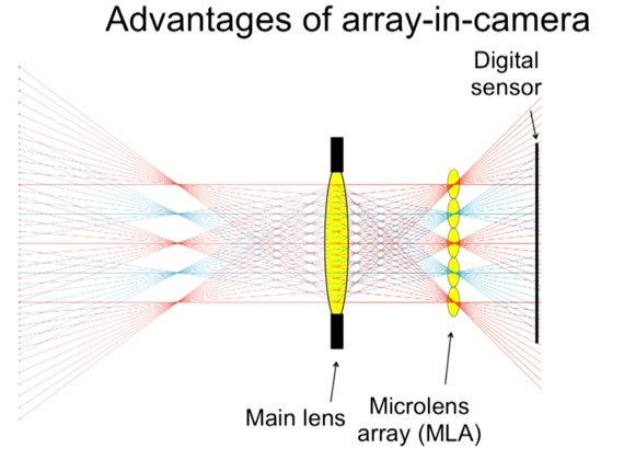
  • A microlens array separates light arriving from different directions.
  • A light field can be reorganized into many slightly offset sub-aperture views.
  • This is similar to capturing the scene from many nearby viewpoints.
• Key Idea
  • Multi-view uses multiple viewpoints to capture parallax.
  • Light fields capture spatial and angular light information more densely.
  • Both can represent 3D structure without explicitly storing geometry.
• Pros
  • Single-shot capture of multiple viewpoints or angular information (Light Field only).
  • High visual fidelity, including view-dependent appearance.
  • Supports computational re-focusing.
  • Can be converted into other representations, such as depth maps, novel views, or 3D geometry.
• Cons
  • High data volume because many views or light-ray samples must be stored.
  • Light Field capture may require specialized camera hardware.
  • Direct Light Field viewing may require specialized display hardware.
  • Spatial or angular resolution can be limited because sensor resolution is shared across multiple views.

Light Field Re-focusing

• Light Field Capture
  • Light field cameras capture light from multiple directions using a microlens array.
  • A single capture contains many slightly different sub-aperture views.
• Re-focusing
  • Objects at different depths show different amounts of parallax across the views.
  • The views can be shifted so that objects at a selected depth align with each other.
  • Aligned objects become sharp when the views are combined.
  • Objects at other depths remain misaligned and appear blurred.
• Virtual Lens
  • A virtual lens computationally reproduces the focusing behavior of a physical lens.
  • This allows the focus position to be changed after the image has already been captured.
• Depth of Field
  • Depth of field is the range of depths that appear sharp.
  • Light field data can also be used to computationally change the depth of field after capture.

Holography

• Reflect light off an object and record its wavefront as an interference pattern using a reference beam.
• Recording
  • A laser is split into an object beam and a reference beam.
  • The object beam reflects off the object and carries the object's wavefront information.
  • A sensor can measure light intensity, but cannot directly measure phase.
  • The reference beam is combined with the object beam so their phase difference becomes a recordable interference pattern.
• Reconstruction
  • A reconstruction beam is sent through the recorded interference pattern.
  • The hologram reconstructs the original wavefront, making the object appear in 3D.
• Holography does not directly encode the object's geometry.
  • It encodes the structure of light reflected from the object.
• Pros
  • Physically accurate reconstruction of light rays.
  • No explicit surface reconstruction required.
  • Quick capture.
• Cons
  • High data volume.
  • Requires a stable coherent light source, usually a laser.
  • Difficult to capture colour and large scenes.
  • Holographic display hardware is expensive and complex.
  • Software reconstruction and post-processing are complex.
• Application
  • Digital Holographic Microscopy (DHM) can reconstruct 3D structures such as red blood cells.

                     Object
                       ↓
Laser → Beam splitter ─────→ Object beam
          │                  ↓ 반사
          │                  ↓
          └────────────→ Reference beam
                             ↓
                    [ Recording plate ]
                       두 빛이 만남
                             ↓
                   Interference pattern

Plenoptic Function

$L(x, y, z, \theta, \phi, \lambda, t)$

• Models the intensity of every light ray in space and time
• $(x, y, z)$: Spatial position
• $(\theta, \phi)$: Viewing direction
• $\lambda$: Wavelength (color)
• $t$: time

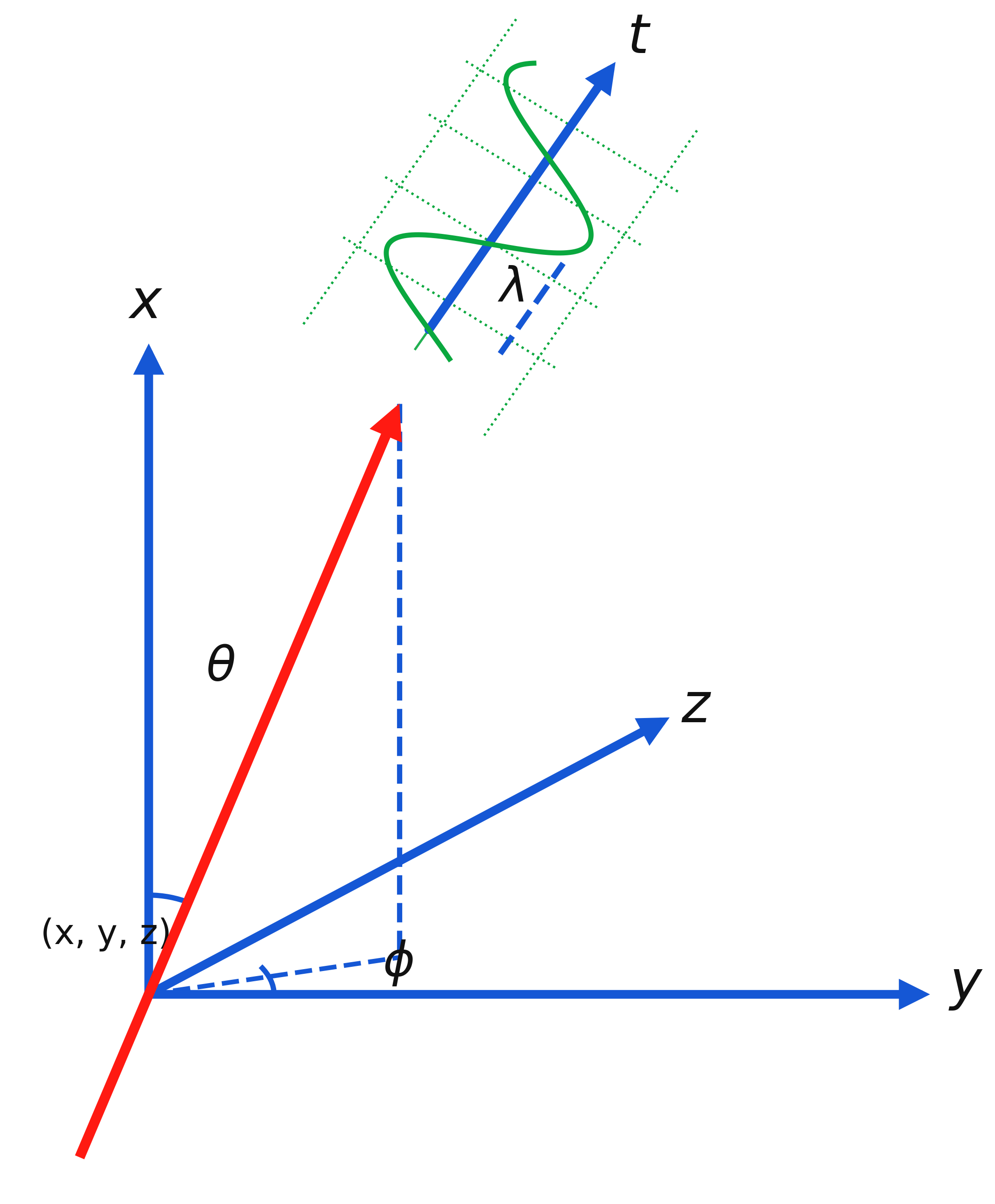
• For human vision, wavelength information can be integrated into RGB channels:
  • $L_R(x, y, z, \theta, \phi,)$
  • $L_G(x, y, z, \theta, \phi,)$
  • $L_B(x, y, z, \theta, \phi,)$
• If only a static image is needed, time can be fixed.
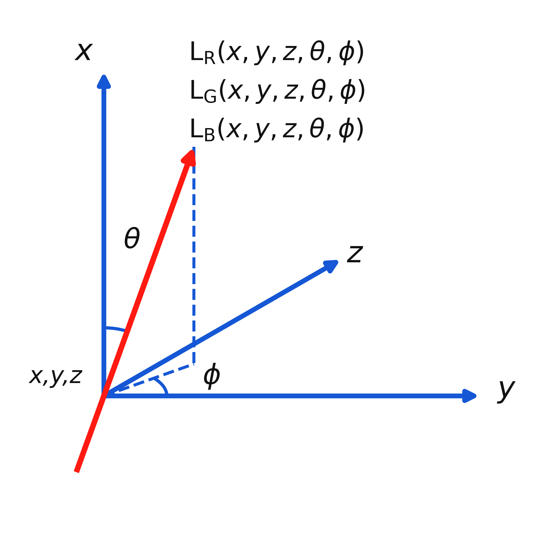
• x, y, z specify the position of the light ray.
• $\theta, \phi$ specify its direction.
• The resulting function describes the RGB light traveling in a particular direction at a particular 3D position.
• This reduces the representation to a 5D spatial-directional function for each RGB channel.
  • space 3D + direction 2D + wavelength 1D (Compressed to RGB) + time 1D (Fixed)

How Cameras Represent the Plenoptic Function

A camera image = integration of rays from the plenoptic function over all directions focused by a lens.

• A camera samples the scene at discrete sensor pixels.
• Multiple rays arriving at each pixel are integrated into a single pixel value.
  • The lens and aperture control which range of rays reaches the pixel.
• Directional information is therefore mostly lost after the rays are integrated.
• Adjusting the lens can change the range of integrated rays, affecting focus and depth of field.

How Light Fields Represent the Plenoptic Function

A light field image = discrete sampling of rays from the plenoptic function over preset directions focused by a lens.

• A light field also samples the scene at discrete sensor positions.
• Instead of integrating different ray directions, it samples them separately.
• A microlens array separates incoming rays according to their directions.
  • Different directions are recorded by different sensor pixels/subpixels.
• Camera arrays and lenslet arrays can collect similar multi-view/angular information.
• More angular sampling provides more directional information, but increases data volume and reduces available spatial resolution.
• Key difference
  • Normal camera: multiple directions → integration → one pixel value.
  • Light field: multiple directions → separate directional samples.

Radiance Fields

래디언스 필드

Representation	Spatial information	Direction information	Result
Traditional camera	x, y	Integrated / collapsed	2D image
Light field	x, y	θ, φ sampled separately	4D image
Radiance field	x, y, z	θ, φ modelled continuously	5D function

• Traditional cameras
  • Integrate multiple incoming ray directions into each pixel.
  • Directional information is collapsed.
  • Result: 2D image
    • I(x, y)
• Light field imaging
  • Samples incoming rays separately over multiple directions.
  • Preserves angular information.
  • Result: 4D light field
    • $L(x, y, \theta, \phi)$
• Radiance field
  • Describes light at each 3D position and viewing direction.
  • $L(x, y, z, \theta, \phi)$ → RGB
  • Conceptually extends light-field modelling from a camera plane into 3D space.
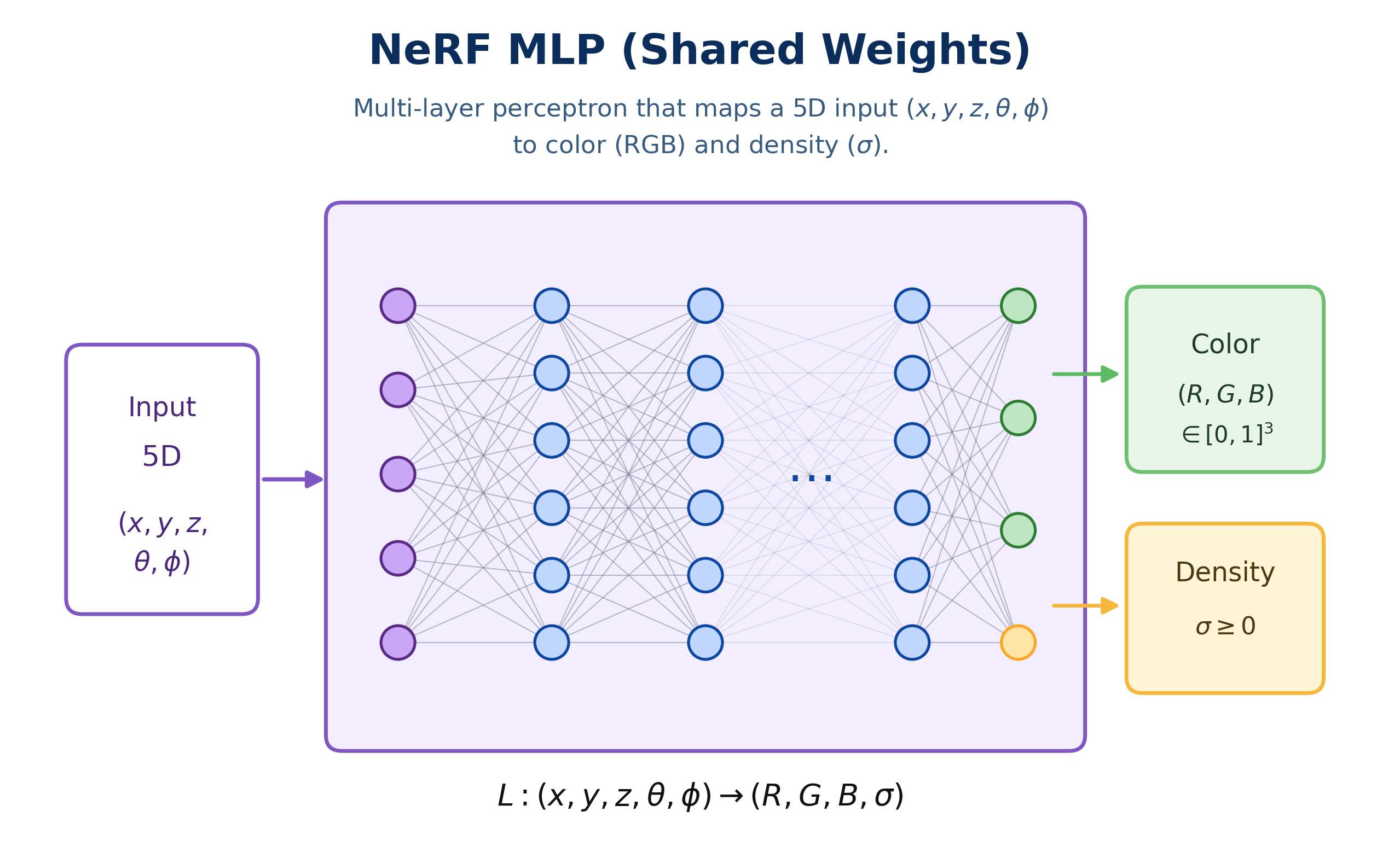
• NeRF
  • Learns the radiance field using a neural network.
  • Input:
    • $x, y, z, \theta, \phi$
  • Output:
    • RGB
    • density $\sigma$
• 3D Gaussian Splatting
  • Uses explicit Gaussian primitives instead of an MLP.
  • Adjusts position, scale, orientation, colour, opacity, etc. to represent the scene and its view-dependent appearance.
• Conceptual shift
  • Geometry modelling → where the object is.
  • Radiance field modelling → what light is seen from each 3D position and direction.

Modern 3D Representations

NeRFs

Neural Radiance Fields

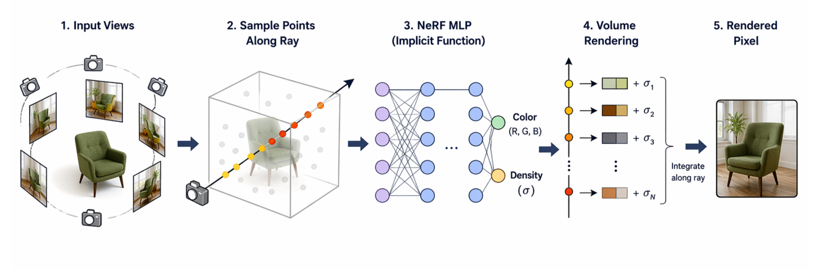
• Light field at any point in space stored in neural network weights.
• Trained from posed images, produces photorealistic novel views.
  • Each image has a known camera position and viewing direction.
• Rendering
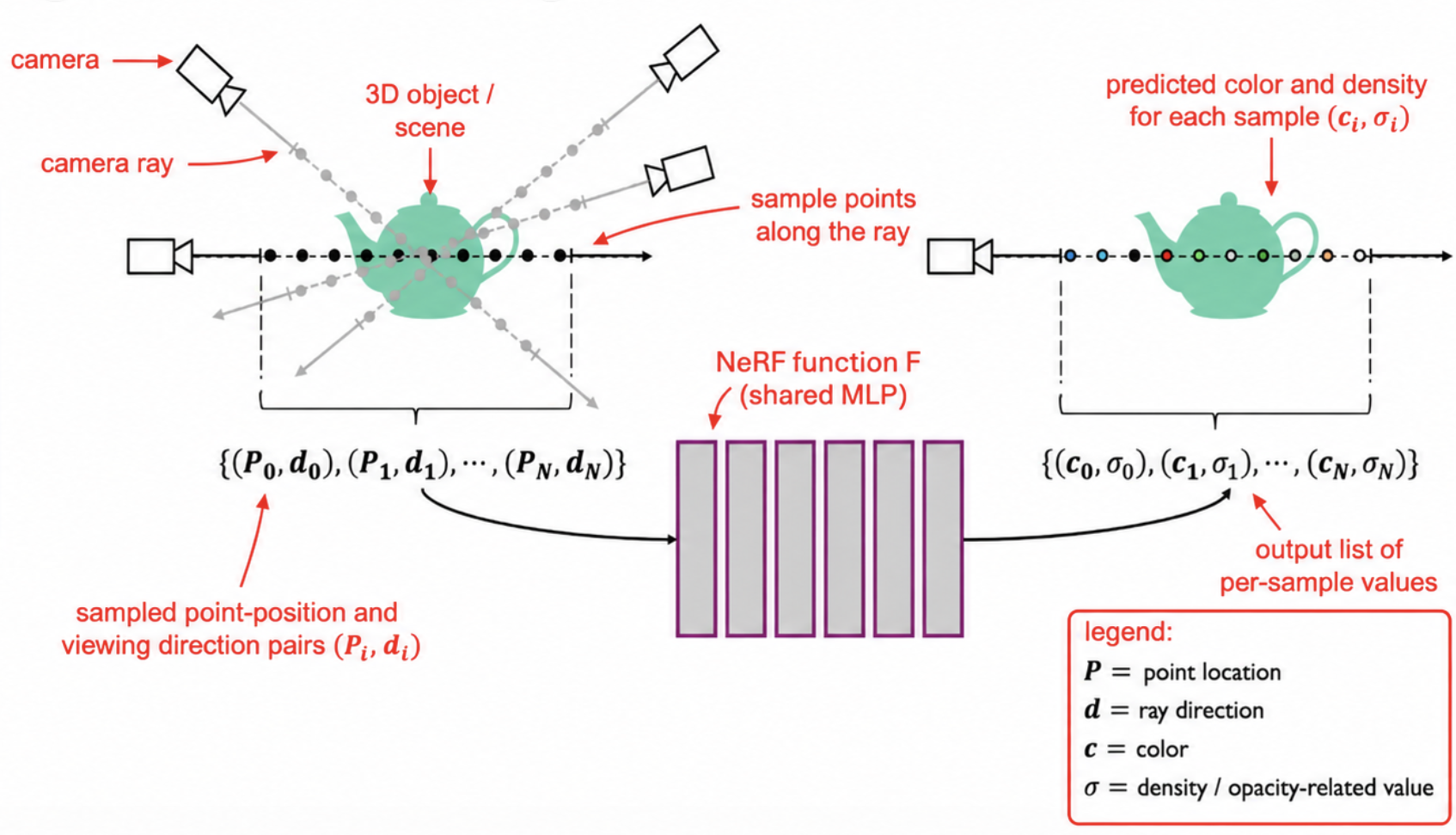
  • Cast a camera ray through each image pixel.
  • Sample multiple 3D points along the ray.
  • Query the NeRF at each point to obtain color and density.
  • Empty points have low density and contribute little.
  • High-density points contribute more and can occlude points behind them.
  • Integrate the weighted colors along the ray to produce one 2D pixel.
• NeRF Studio

• Pros:
  • High photorealism/fidelity
  • Continuous scene representation
  • View-dependent effects
  • Data-efficient capture
  • Unified geometry and appearance encoding
• Cons:
  • High computational cost
  • Slow training and rendering
  • Poor scalability
  • Entangled Geometry, appearance and rendering.

Gaussian Splatting

Aspect	Point Clouds	3D Gaussian Splatting (3DGS)
Spatial position	Yes	Yes
Color	RGB, if available	RGB
Opacity	None	Yes
Scale	None	Yes
Orientation	None	Yes
Color directionality	None	Yes; color can vary by viewing direction

• Instead of building objects using polygons, it represents everything using millions of tiny soft 3D shapes called Gaussians.
  • Represent scenes explicitly as a collection of Gaussian primitives, optimized directly for efficient and accurate rendering.
• Initialization steps:
  • Initialize point clouds
  • Find central point of 3D Gaussians.
  • A covariance matrix containing shape information is calculated.
  • Added opacity to each 3D Gaussians.

1. First, it builds a rough point cloud from images
2. Then, replaces those points with these Gaussian blobs
3. It will optimize them until it match original photos as closely as possible.

• Pros:
  • Realtime rendering at interactive frame rates.
  • High-quality visual outputs with detailed textures.
  • Efficient and compact representation compared to implicit methods.
• Cons:
  • View-dependent quality degradation: rendering quality varies significantly across different viewing angles, causing inconsistency in visual outputs.
  • Sensitivity to initialization: final rendering quality heavily depends on initial placement of Gaussians, impacting optimization stability.
  • Inefficient Gaussian distribution: Fixed-scale Gaussians may fail to adapt effectively across scenes with varying geometric complexity.

Aspect	NeRF	3D Gaussian Splatting (3DGS)
Representation	Implicit MLP representation	Explicit set of Gaussian primitives
Rendering	Ray sampling and volume integration	Rasterization and splatting
Training	Optimize network weights	Directly optimize scene parameters
Sampling	Dense sampling along each ray	No dense per-ray sampling
Rendering speed	Slower	Fast / real-time rendering

Applications of 3D Representations

• Immersive Interaction and Communication
  • Real-world scene integration in extended reality environments
  • Telepresence and virtual communication
    • Telehealth experiences for remote consultations
  • Digital cinematography and VFX
  • Retail and virtual try-on
  • Immersive storytelling for news and events
  • Computer graphics and gaming
• Spatial Analysis and Operational Environments
  • Simulation and navigation for autonomous systems
  • AEC (Architecture, Engineering, and Construction)
  • Industrial imaging
  • GIS (Geographic Information Systems) Inspection and Mapping
• Scientific Visualization and Digital Heritage
  • Cultural heritage digitization
  • Medical imaging
  • Scientific modeling
  • Fluid simulation