RL 001

Reinforcement Learning

• Learn how to make a good sequence of decisions by interacting with the environment.

Characteristics of RL

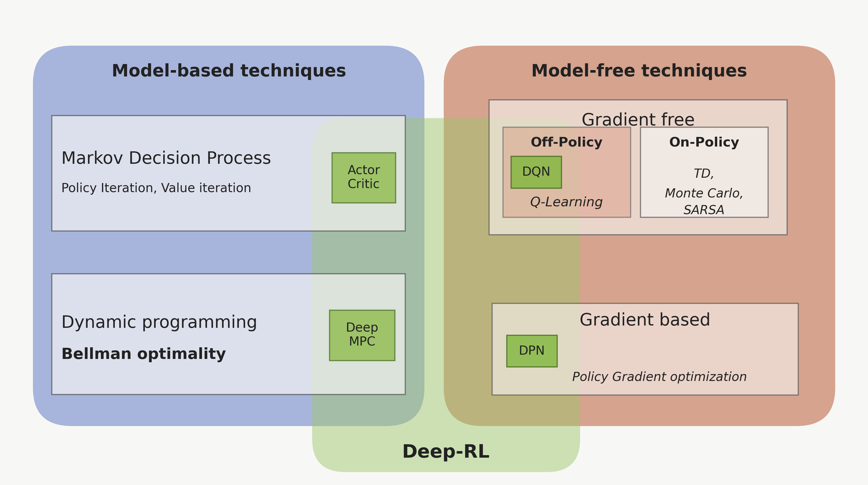
• Trial and Error: Based learning approach.
• Optimization: Find good sequences of actions or decisions.
• Delayed Consequences/Rewards: Takes time to relize the actions or decisions are good or bad.
• Exploration: Learn by making decisions or forming actions or through experiences. Trying new actions to discover their effects.
• Exploitation: Choosing actions with the highest expected reward, based on current knowledge.
• Generalization: Use previous experiences or knowledge to new or unseen situations effectively.

Framwork of RL

• OpenAI Gym
• Torch RL
• AWS DeepRacer

RL Math

Probability

• Sample Space ($\Omega$): The set of all possible outcomes of a random experiment.

Bonferroni's Inequality

$P(A \cap B) \geq P(A) + P(B) - 1$ $P(\cap^{n}_{i=1} A_i) \geq \sum_{i=1}^{n} P(A_i) - (n-1)$

• Gives a lower bound on the intersection probability which is useful when this probability is difficult to compute directly.
• It is useful when the probabilities of individual events are sufficiently large.

Boole's Inequality

$P(\cup^{n}_{i=1} A_i) \leq \sum_{i=1}^{n} P(A_i)$

for any sets $A_1, A_2, ..., A_n$.

• It is useful when finding an upper bound for the probabilities of the union of events.

Bayes' Rule

$P(A|B) = \frac{P(A \cap B)}{P(B)}$ $P(A\cap B) = P(B|A) P(A) = P(A|B) P(B)$ $P(A|B)P(B) = P(B|A)P(A)$ $P(A|B) = \frac{P(B|A) P(A)}{P(B)}$

• It allows us to compute the conditional probability $P(A|B)$ from the inverse conditional probability $P(B|A)$.
• Let $A_1, A_2, ..., A_n$ be a partition of the sample space $S$. Then let $B$ be any subset of $S$ we have:

$P(A_i|B) = \frac{P(B|A_i) P(A_i)}{\sum_{j=1}^{\infty} P(B|A_j) P(A_j)}$

Independent Events

$P(A \cap B) = P(A) P(B)$

• A family $A_i :i \in I$ of events is independent if for every finite subset $J \subseteq I$ we have: $P\left(\bigcap_{i \in J} A_i\right) = \prod_{i \in J} P(A_i)$

• The pair-wise independence of events does not imply their mutual independence.

Conditional Independence

$P(A \cap B|C) = P(A|C) P(B|C)$

• where $P(C) > 0$.
• or equivalently, $P(A|B \cap C) = P(A|C)$ and $P(B|A \cap C) = P(B|C)$.

Induced Probability Function

$P_X(x_i) = P\big(\{w_j \in \Omega : X(w_j) = x_i\}\big)$

• $\Omega = \{w_1, w_2, ..., w_m\}$ is the sample space.
• $X$ is a random variable with range $X = \{x_1, x_2, ..., x_n\}$.
• The result set $\{w_j \in \Omega : X(w_j) = x_i\}$ is the set of all outcomes in the sample space that map to the value $x_i$ under the random variable $X$.

Cumulative Distribution Function (CDF)

$F_X(x) = P_X(X \leq x) \quad \forall x \in \mathbb{R}$

• $F_X(x)$ is a cdf $\iff$ the following conditions hold:
  • Monotonicity: $F_X(x)$ is non-decreasing.
  • Limiting values: $\lim_{x \to -\infty} F_X(x) = 0$ and $\lim_{x \to \infty} F_X(x) = 1$.
  • Right-Continuity: $\lim_{y \downarrow x} F_X(y) = F_X(x) \quad \forall x \in \mathbb{R}$.

F_X(t)

1.0 |                         ●────────────
    |                         ↑  ↑  ↑
    |                      3.001 3.01 3.1
0.7 |              ●─────────○
    |              ↑  ↑  ↑
    |           2.001 2.01 2.1
0.3 |     ●────────○
    |     ↑  ↑  ↑
    |  1.001 1.01 1.1
0.0 |─────○
    +-------------------------------------- t
          1         2         3
          x         x         x

Continuous & Discrete Random Variables

• if $X$ is continuous, then $F_X(x)$ is continuous and differentiable almost everywhere. The probability density function (pdf) is defined as: $f_X(x) = \frac{d}{dx} F_X(x)$
• if $X$ is discrete, then $F_X(x)$ is a step function and the probability mass function (pmf) is defined as: $p_X(x_i) = P(X = x_i)$

1 ────────────────────────━━━━━━━━
                        ╱
                      ╱
                    ╱
                  ╱
0 ━━━━━━━━━━━━━━━───────────────── x

1 ─────────────────────────●━━━━━━
                           │
0.7 ─────────────●━━━━━━━━━○
                 │
0.3 ─────●━━━━━━━○
         │
0 ━━━━━━━○──────────────────────── x
         1         2         3

1 ──────────────────────────━━━━━━
                          ╱
                        ╱
0.7 ───────────●━━━━━━━
               │
0.5 ───────────○
             ╱
           ╱
0 ━━━━━━━━──────────────────────── x
               a

Probability Mass Function (PMF)

$$f_X(x)= \begin{cases} (1-p)^{x-1}p, & x=1,2,3,\ldots \\ 0, & \text{otherwise} \end{cases}$$

• A discrete random variable $X$ is given by $f_X(x) = P(X=x)$ for $x \in \mathbb{R}$.
• It represents the probability that the first success occurs exactly on the $x$-th trial in a sequence of independent trials.

Probability Density Function (PDF)

$$F_X(x) = \int_{-\infty}^{x} f_X(t) dt \quad \forall x \in \mathbb{R}$$

• A continuous random variable $X$ is given by $f_X(x)$ for $x \in \mathbb{R}$.
• The probability is calculated as the area under the probability density function over a specific interval.

Expectation

$E[X] = \sum x P(X=x) \quad \text{if } X \text{ is discrete}$

$E[X] = \int_{-\infty}^{\infty} x f_X(x) dx \quad \text{if } X \text{ is continuous}$

• Linearity: $E[aX + bY + c] = aE[X] + bE[Y] + c$ for any constants $a$, $b$, and $c$.
• Non-negativity: If $X \geq 0$ then $E[X] \geq 0$ because it is a weighted average of non-negative values.
• Monotonicity: If $X \geq Y$ then $E[X] \geq E[Y]$ because it is a weighted average of values that are greater than or equal to the corresponding values of $Y$.
• Boundedness: If $a \leq X \leq b$ then $a \leq E[X] \leq b$ because it is a weighted average of values that are bounded by $a$ and $b$.

a ●──────────────●──────────────● b
       가능한 값들    평균
                   E[X]

Moments

$\mu'_n = E[X^n] \quad \forall n \in \mathbb{N}$

• The $n^{th}$ central moment of $X$ is: $\mu_n = E[(X - E[X])^n] = E(X - \mu)^n$

• 1th central moment is the mean, $\mu_1 = E[X]$.

• 2th central moment is the variance, $\mu_2 = E[(X - E[X])^2] = \text{Var}(X)$.

  • It emphasizes the variability of the distribution.
  • $\text{Var}(aX + b) = a^2 \text{Var}(X)$ for any constants $a$ and $b$.

• 3th central moment is the skewness, $\mu_3 = E[(X - E[X])^3]$.

  • It emphasizes the skewness of the distribution.

• 4th central moment is the kurtosis, $\mu_4 = E[(X - E[X])^4]$.

  • It emphasizes the tail behavior and extreme values of the distribution.

Covariance

$\text{cov(X, Y)} = E[(X - E[X])(Y - E[Y])]$

• It measures how muc htwo random variables change together.
• Negative Covariance
• Near Zero Covariance
• Positive Covariance

Y: 시험 점수

높음  |                ●
     |          ●  ●
     |       ●
     |    ●
낮음  | ●
     +-------------------- X: 공부 시간
       적음             많음

       Cov(X,Y) > 0

Correlation

$p(X, Y) = \frac{\text{cov(X, Y)}}{\sqrt{\text{Var}(X)\text{Var}(Y)}}$

• Individual variances must be non-zero.
• $p(X, Y)$ lies in the range $[-1, 1]$.

Joint Distributions

$f_{X,Y}:\mathbb{R}^2\to[0,1], \\ f_{X,Y}(x,y) = P(X=x, Y=y) \quad \text{if } X, Y \text{ are discrete}$

• Joint Probability Mass Function (PMF) for discrete random variables $X$ and $Y$.

Y
1 ┤  ● 1/4       ● 1/4
  │ (0,1)       (1,1)
0 ┤  ● 1/4       ● 1/4
  │ (0,0)       (1,0)
  └──────────────────── X
      0           1

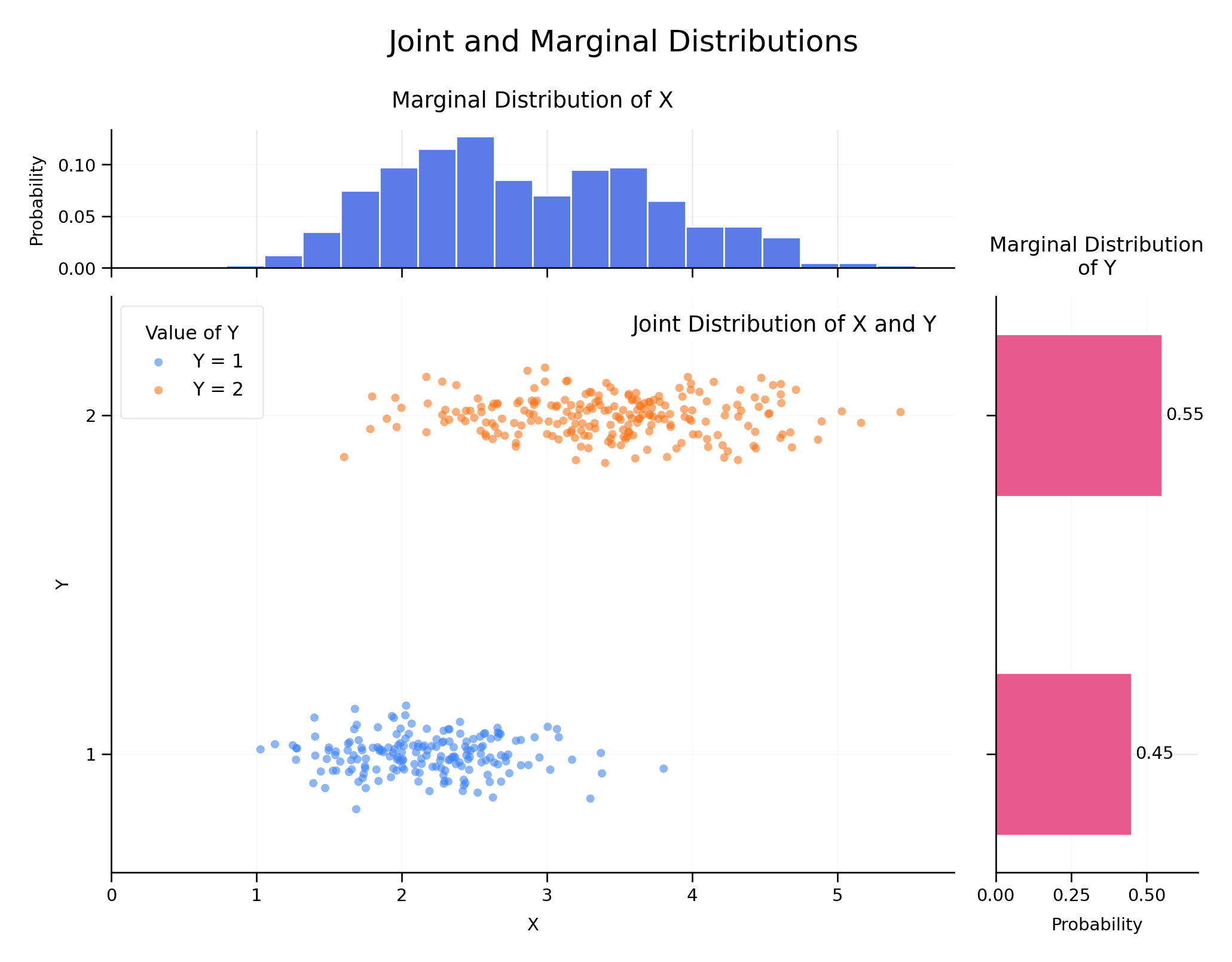
Marginal Distributions

$f_X(x) = \sum_{y} f_{X,Y}(x,y) \\ f_Y(y) = \sum_{x} f_{X,Y}(x,y)$

• Fixing one variable and summing over the other variable gives the marginal distribution of the fixed variable.

             Y=0       Y=1       행의 합
X=0          0.10      0.20        0.30
X=1          0.30      0.40        0.70
             ─────────────────────────
열의 합       0.40      0.60        1.00

• $f_X(0) = 0.10 + 0.20 = 0.30$: sum of the first row.
• $f_X(1) = 0.30 + 0.40 = 0.70$: sum of the second row.
• $f_Y(0) = 0.10 + 0.30 = 0.40$: sum of the first column.
• $f_Y(1) = 0.20 + 0.40 = 0.60$: sum of the second column.
• Marginalization: It sums or integrates over all possible values of an unwanted variable to obtain the distribution of the variable of interest.

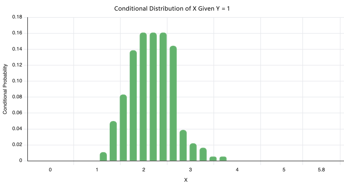
Conditional Distributions

$f_{X|Y}(x|y) = P(X = x | Y = y) = \frac{f_{X,Y}(x,y)}{f_Y(y)} \quad \text{if } f_Y(y) > 0$

• It represents the probability distribution of $X$ given that $Y$ has a specific value.
• If $f_Y(y) = 0$, then $f_{X|Y}(x|y)$ is undefined.

Bernoulli Distribution

$X = \begin{cases} 1, & \text{with probability } p \\ 0, & \text{with probability } 1-p \end{cases}$

• $E[X] = p$
• $\text{Var}(X) = p(1-p)$
• The outcome of a Bernoulli trial is either a success (1) or a failure (0).

Binomial Distribution

• probability of success in a single trial: $p$
• probability of failure in a single trial: $q = 1 - p$

$P(X = x|n, p) = \binom{n}{x} p^x q^{n-x} \\ \text{where} \binom{n}{x} = \frac{n!}{x!(n-x)!}, \quad 0 \leq x \leq n$

• $E[X] = np$
• $\text{Var}(X) = npq = np(1-p)$
• The binomial distribution describes the number of successes in a fixed number of independent Bernoulli trials.
• $X \sim \text{Binomial}(10, 0.7)$
  • $P(X = 7) = \binom{10}{7} (0.7)^7 (0.3)^3 \approx 0.2668$

Geometric Distribution

• probability of success in a single trial: $p$
• probability of failure in a single trial: $q = 1 - p$

$P(X = x|p) = (q^{x-1}) p \\ \text{where } x = 1, 2, 3, ...$

• $E[X] = \frac{1}{p}$
• $\text{Var}(X) = \frac{q}{p^2}$
• The geometric distribution describes the number of trials before the first success in a sequence of independent Bernoulli trials.
• $X \sim \text{Geometric}(0.7)$
  • $P(X = 3) = (0.3)^2 (0.7) \approx 0.063$

Uniform Distribution

$f_X(x|a,b) = \begin{cases} \frac{1}{b-a}, & a \leq x \leq b \\ 0, & \text{otherwise} \end{cases}$

• $E[X] = \frac{a+b}{2}$
• $\text{Var}(X) = \frac{(b-a)^2}{12}$
• The uniform distribution describes a continuous random variable that has an equal probability of taking any value within a specified range.
• The probability depends on the length of the interval, not its location.

Normal Distribution

$f_X(x) = \frac{1}{\sqrt{2\pi\sigma^2}} e^{-\frac{(x-\mu)^2}{2\sigma^2}}, \quad -\infty < x < \infty$

$X \sim N(\mu, \sigma^2)$

• Central Limit Theorem: the distribution of the sum (or average) of a large number of independent, identically distributed variables will be approximately normal, regardless of the underlying distribution.

$\bar{X} = \frac{1}{n} \sum_{i=1}^{n} X_i \approx N\left(\mu, \frac{\sigma^2}{n}\right)$

Multivariate Normal Distribution

$N(x|\mu, \Sigma) = \frac{1}{\sqrt{(2\pi)^D |\Sigma|}} e^{-\frac{1}{2} (x-\mu)^T \Sigma^{-1} (x-\mu)}$

• $\mu$ is the $D$-dimensional mean vector.
• $\Sigma$ is the $D \times D$ covariance matrix.
• $|\Sigma|$ is the determinant of the covariance matrix.

Beta Distribution

$f(x|\alpha, \beta) = \frac{\Gamma(\alpha + \beta)}{\Gamma(\alpha)\Gamma(\beta)} x^{\alpha - 1} (1 - x)^{\beta - 1}, \quad 0 < x < 1$

• $\Gamma(n) = (n-1)!$ is the gamma function.
• $E[X] = \frac{\alpha}{\alpha + \beta}$
• $\text{Var}(X) = \frac{\alpha \beta}{(\alpha + \beta)^2 (\alpha + \beta + 1)}$

α < β                  α = β                  α > β

높이                   높이                   높이
│╲                     │    ╭──╮             │        ╱
│ ╲___                 │  ╭─╯  ╰─╮           │    ___╱
└──────── x            └────────── x         └──────── x
0        1             0          1           0        1

0 쪽 강조              가운데 강조             1 쪽 강조

Beta(8,2)                 Beta(80,20)

       ╭────╮                    /\
     ╭─╯    ╰─╮                 /  \
─────╯        ╰───        ─────/────\─────
         0.8                      0.8

불확실성 큼                 불확실성 작음

• $p | \text{data} \sim \text{Beta}(\alpha + s, \beta + f)$
  • where new observations are $s$ successes and $f$ failures.
• The Beta distribution is a distribution of success probabilities for a Bernoulli or Binomial distribution.
• Application
  • Measuring uncertainty in the probability of success for a Bernoulli or Binomial distribution.
  • Conversion rate or click-through rate (CTR) in online advertising.
  • Defect rate in manufacturing.

Linear Algebra

Axioms of Vector Spaces

• Commutative Law: $u + v = v + u, \quad \forall u, v \in V$
• Associative Law: $(u + v) + w = u + (v + w), \quad \forall u, v, w \in V$
• Additive Identity: $\exists 0 \in V$ such that $v + 0 = v, \quad \forall v \in V$
• Additive Inverse: $\forall v \in V, \exists -v \in V$ such that $v + (-v) = 0$
• Distributive Law:
  • $a(u + v) = au + av, \quad \forall a \in F, u, v \in V$
  • $(a + b)v = av + bv, \quad \forall a, b \in F, v \in V$
• Associative Law: $(ab)v = a(bv), \quad \forall a, b \in F, v \in V$
• Unitary Law: $1v = v, \quad \forall v \in V$

Subspace

• $x + \alpha y \in W, \quad \forall x, y \in W, \forall \alpha \in \mathbb{R}$

Norm

$f: \mathbb{R}^n \to \mathbb{R}$

• It outputs a real number that represents the length or size of a vector in a vector space.

$x=(x_1,x_2,\ldots,x_n) \mapsto f(x)=\lVert x\rVert$

• Non-negativity: $\forall x \in \mathbb{R}^n, \quad \lVert x\rVert \geq 0$
• Definiteness: $f(x) = 0 \iff x = 0$
• Homogeneity: $\forall x \in \mathbb{R}^n, \quad \forall t \in \mathbb{R}, f(tx) = |t| f(x)$
• Triangle inequality: $\forall x,y \in \mathbb{R}^n, \quad f(x+y) \leq f(x) + f(y)$
  • $\lVert x + y \rVert \leq \lVert x \rVert + \lVert y \rVert$
• A norm is non-negative, only the zero vector has a norm of zero, scaling a vector by two doubles its norm, and the direct distance cannot be greater than the detoured distance.

$\lVert x \rVert_p = (\sum_{i=1}^{n} |x_i|^p)^{\frac{1}{p}}, \quad p \geq 1$

• L1 norm: $\lVert x \rVert_1 = \sum_{i=1}^{n} |x_i|$
  • Manhattan distance.
• L2 norm: $\lVert x \rVert_2 = \sqrt{\sum_{i=1}^{n} |x_i|^2}$
  • Euclidean distance.
• L-infinity norm: $\lVert x \rVert_\infty = \max_i|x_i|$
  • $\lVert (3, 4) \rVert_\infty = \max\{3, 4\} = 4$

$\lVert A \rVert_F = \sqrt{\sum_{i=1}^{m} \sum_{j=1}^{n} |a_{ij}|^2} = \sqrt{\text{tr}(A^T A)}$

• Frobenius norm: $A = \begin{bmatrix} 1 & 2 \\ 3 & 4 \end{bmatrix}$
  • $\lVert A \rVert_F = \sqrt{1^2 + 2^2 + 3^2 + 4^2} = \sqrt{30}$
  • It is the square root of the sum of the absolute squares of its elements.

Span

$span\{x_1, x_2, ..., x_n\} = \{ \alpha_1 x_1 + \alpha_2 x_2 + ... + \alpha_n x_n : \alpha_n \in \mathbb{R}\}$

• A set of vertors $X = \{x_1, x_2, ..., x_n\}$ in a vector space $V$ is said to span $V$ if every vector in $V$ can be expressed as a linear combination of the vectors in $X$.
• Span is the entire region that can be reached by scaling and adding the given vectors.

Range

$R(A) = \{\alpha_1 a_1 + \alpha_2 a_2 + ... + \alpha_n a_n : \alpha_n \in \mathbb{R}\}$

• The range of a matrix $A$ is the set of all possible linear combinations of its column vectors.
• Same as the columnspace of the matrix $A$.

Nullspace

$N(A) = \{x \in \mathbb{R}^n : Ax = 0\}$

• A set of all vectors that equal 0 when multiplied by the matrix $A$.
• The dimensionality of the nullspace is called the nullity of the matrix $A$.

Linear Independence

• A set of vectors $\{v_1, v_2, ..., v_n\}$ is said to be linearly independent if the only solution to the equation $\alpha_1 v_1 + \alpha_2 v_2 + ... + \alpha_n v_n = 0$ is $\alpha_1 = \alpha_2 = ... = \alpha_n = 0$.
• Column rank: The maximum number of linearly independent column vectors in a matrix.
• Row rank: The maximum number of linearly independent row vectors in a matrix.
• If one row vector is a combination of other row vectors, then it is linearly dependent.
• The number of rows that are removed due to redundancy is the Rank of the matrix.
• Due to the redundancy, the number of directions which is vanishing is the Nullity of the matrix.

Rank

$Rank(A) = \text{dim}(R(A)), \quad A \in \mathbb{R}^{m \times n}$

• $rank(A) \leq \min(m, n), \quad A \in \mathbb{R}^{m \times n}$
  • if $rank(A) = min(m, n)$, then $A$ is said to be full rank.
  • Rank cannot exceed the number of rows or columns in the matrix.
• $rank(A) = rank(A^T), \quad A \in \mathbb{R}^{m \times n}$
  • The rank of a matrix is equal to the rank of its transpose.
  • The amount of independent information in the rows is equal to the amount of independent information in the columns.
• $rank(AB) \leq \min(rank(A), rank(B)), \quad A \in \mathbb{R}^{m \times n}, B \in \mathbb{R}^{n \times p}$
  • The information content of the product of two matrices cannot exceed the information content of either matrix.
• $rank(A + B) \leq rank(A) + rank(B), \quad A, B \in \mathbb{R}^{m \times n}$
  • The information content of the sum of two matrices cannot exceed the sum of the information content of each matrix.

Orthogonal Matrices

$U \in \mathbb{R}^{n \times n} \text{ is orthogonal } \iff v_i^T v_j = \begin{cases} 1 & \text{if } i = j \\ 0 & \text{if } i \neq j \end{cases}$

• $UU^T = U^TU = I_n$
• $\lVert Ux \rVert_2 = \lVert x \rVert_2, \quad \forall x \in \mathbb{R}^n$
• Orthonormal: A set of vectors is orthonormal if they are all unit vectors and orthogonal to each other.
• Rotation: $R(\theta) = \begin{bmatrix} \cos\theta & -\sin\theta \\ \sin\theta & \cos\theta \end{bmatrix}$
• Reflection: $R = \begin{bmatrix} 1 & 0 \\ 0 & -1 \end{bmatrix}$

Quadratic Form

$Q(x) = x^T A x, \quad A \in \mathbb{R}^{n \times n}$

• The quadratic form $x^TAx$ gives a scalar value that measures the cost, energy, or weighted magnitude of the vextor $x$, according to the quadratic surface defined by the matrix $A$.
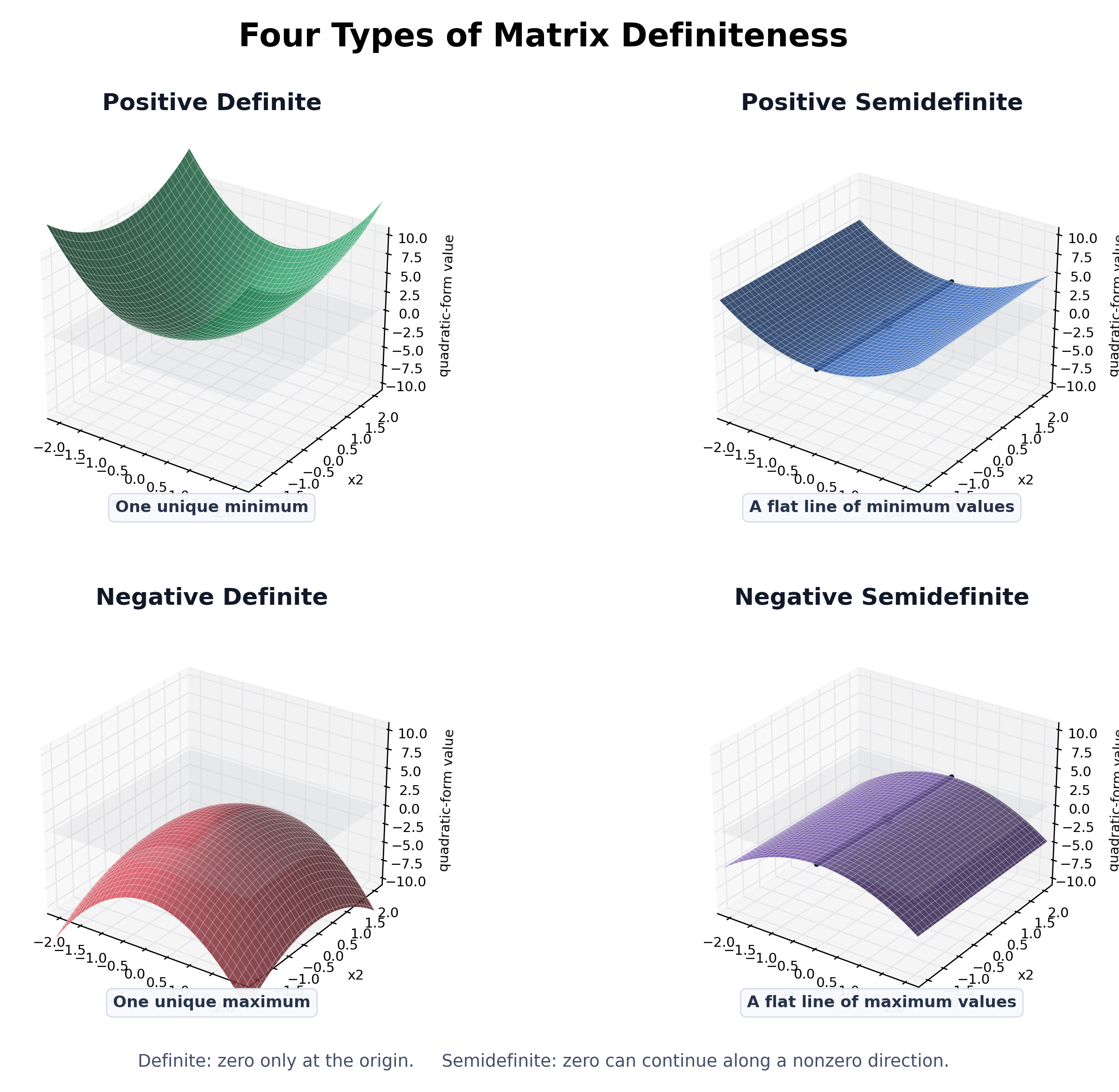
  • Positive definite: $Q(x) > 0, \quad \forall x \neq 0$
  • Positive semi-definite: $Q(x) \geq 0, \quad \forall x \neq 0$
  • Negative definite: $Q(x) < 0, \quad \forall x \neq 0$
  • Negative semi-definite: $Q(x) \leq 0, \quad \forall x \neq 0$
  • Indefinite: $Q(x)$ can be positive or negative for different $x \neq 0$

• 행렬의 정부호성(양의 정부호, 양의 준정부호, 음의 정부호, 음의 준정부호, 부정정부호)

$A^TA = A^TA \implies Q(x) = x^T A^T A x = (Ax)^T (Ax) = \lVert Ax \rVert^2 \geq 0$

• Always positive semi-definite because it is the square of the norm of the vector $Ax$.

Eigenvalues & Eigenvectors

$\lambda \in \mathbb{R} \text{ is an eigenvalue of } A \in \mathbb{R}^{n \times n} \iff A\vec{x} = \lambda \vec{x} , \quad \vec{x} \in \mathbb{R}^n, \vec{x} \neq 0$

• An eigenvector is a nonzero vector that remains on the same line when transformed by a matrix.
• Its eigenvalue tells us how much the vector is scaled and whether its direction is reversed.

$\text{det}(A - \lambda I) = 0$

• $A = \begin{bmatrix} 4 & 1 \\ 2 & 3 \end{bmatrix}$
• $A - \lambda I = \begin{bmatrix} 4 - \lambda & 1 \\ 2 & 3 - \lambda \end{bmatrix}$
• $\text{det}(A - \lambda I) = (4 - \lambda)(3 - \lambda) - 2 = \lambda^2 - 7\lambda + 10 = (\lambda - 5)(\lambda - 2) = 0$
• $\lambda_1 = 5, \quad \lambda_2 = 2$

$\text{tr}(A) = \sum_{i=1}^{n} \lambda_i$

• The trace is the sum of the scaling factors along all eigenvector directions.

$\text{det}(A) = \prod_{i=1}^{n} \lambda_i$

• The determinant is the product of the eigenvalues, representing the overall signed scaling factor for area or volume.

$rank(A) = \text{number of non-zero eigenvalues of } A$

• For a diagonalizable matrix, the rank equals the number of nonzero eigenvalues, counted with multiplicity.

$\lambda_i (A^{-1}) = \frac{1}{\lambda_i(A)}$

• The eigenvalues of the inverse of a matrix are the reciprocals of the eigenvalues of the original matrix.

$A \vec{x} = \lambda \vec{x} \\ \implies A^{-1} A \vec{x} = A^{-1} \lambda \vec{x} \\ \implies \vec{x} = \lambda A^{-1} \vec{x} \\ \implies A^{-1} \vec{x} = \frac{1}{\lambda} \vec{x}$

Diagonalization

$S = \begin{bmatrix} \vdots & \vdots & \cdots & \vdots \\ \vec{v_1} & \vec{v_2} & \cdots & \vec{v_n} \\ \vdots & \vdots & \cdots & \vdots \end{bmatrix}$ $AS = \begin{bmatrix} \vdots & \vdots & \cdots & \vdots \\ \lambda_1\vec{v_1} & \lambda_2\vec{v_2} & \cdots & \lambda_n\vec{v_n} \\ \vdots & \vdots & \cdots & \vdots \end{bmatrix} \\ = \begin{bmatrix} \vdots & \vdots & \cdots & \vdots \\ \vec{v_1} & \vec{v_2} & \cdots & \vec{v_n} \\ \vdots & \vdots & \cdots & \vdots \end{bmatrix} \begin{bmatrix} \lambda_1 & 0 & \cdots & 0 \\ 0 & \lambda_2 & \cdots & 0 \\ \vdots & \vdots & \ddots & \vdots \\ 0 & 0 & \cdots & \lambda_n \end{bmatrix} \\ = S\Lambda$

• $S^{-1}AS = \Lambda$
  • $AS = S\Lambda$
  • $S^{-1}AS = S^{-1}S\Lambda = \mathbb{I}\Lambda = \Lambda$
  • A matrix $A$ that appears complicated in the original coordinate system becomes the diagonal matrix $\Lambda$ when expressed in the eigenvector coordinate system.
• $A = S\Lambda S^{-1}$
  • In the eigenvector basis, the matrix $A$ becomes the diagonal matrix $\Lambda$.

Symmetric Matrices

• A real symmetric matrix satisfies $A=A^T$.
• All eigenvalues of a real symmetric matrix are real.
• A real symmetric matrix has a complete set of orthonormal eigenvectors.
• Therefore, the eigenvector matrix $S$ is orthogonal.

$$S^TS=\mathbb{I} \quad\Longrightarrow\quad S^{-1}=S^T$$

• The diagonalization of a symmetric matrix is

$$A=S\Lambda S^T$$

• $S$ contains the orthonormal eigenvectors of $A$.
• $\Lambda$ contains the corresponding eigenvalues.
• $S^T$ converts $x$ into the eigenvector basis.
• $\Lambda$ scales each eigenvector direction by its corresponding eigenvalue.
• $S$ converts the result back to the original basis.

Definiteness of Symmetric Matrices

• Using $A=S\Lambda S^T$ and $y=S^Tx$,

$$x^TAx = x^TS\Lambda S^Tx = y^T\Lambda y = \sum_{i=1}^{n}\lambda_i y_i^2$$

• $y_i$ is the component of $x$ along the $i$-th eigenvector.

• Since $y_i^2\geq0$, the sign of $x^TAx$ depends entirely on the signs of the eigenvalues.

• If all eigenvalues are positive, $A$ is positive definite.

$$\lambda_i>0\text{ for all }i \quad\Longrightarrow\quad x^TAx>0\text{ for all }x\neq0$$

• If all eigenvalues are non-negative, $A$ is positive semidefinite (PSD).

$$\lambda_i\geq0\text{ for all }i \quad\Longrightarrow\quad x^TAx\geq0$$

• If all eigenvalues are negative, $A$ is negative definite.

$$\lambda_i<0\text{ for all }i \quad\Longrightarrow\quad x^TAx<0\text{ for all }x\neq0$$

• If all eigenvalues are non-positive, $A$ is negative semidefinite (NSD).

$$\lambda_i\leq0\text{ for all }i \quad\Longrightarrow\quad x^TAx\leq0$$

• If $A$ has both positive and negative eigenvalues, $A$ is indefinite.
• The eigenvectors determine the principal directions of the quadratic surface.
• The eigenvalues determine the curvature and sign along those directions.
• The definiteness of a symmetric matrix is determined entirely by the signs of its eigenvalues.

Eigenvalues of a Positive Semidefinite Matrix

• If $A$ is positive semidefinite, then

$$x^TAx\geq0$$

• For an eigenvector $\vec{x}\neq\vec{0}$ with eigenvalue $\lambda$,

$$A\vec{x}=\lambda\vec{x}$$ $$\vec{x}^{\,T}A\vec{x} = \vec{x}^{\,T}(\lambda\vec{x}) = \lambda\vec{x}^{\,T}\vec{x} = \lambda\lVert\vec{x}\rVert^2 \geq0$$

• Since $\vec{x}\neq\vec{0}$,

$$\lVert\vec{x}\rVert^2>0$$

• Therefore,

$$\lambda\geq0$$

• Hence, all eigenvalues of a positive semidefinite matrix are non-negative.
• A zero eigenvalue means that the corresponding eigenvector direction is collapsed to the zero vector.

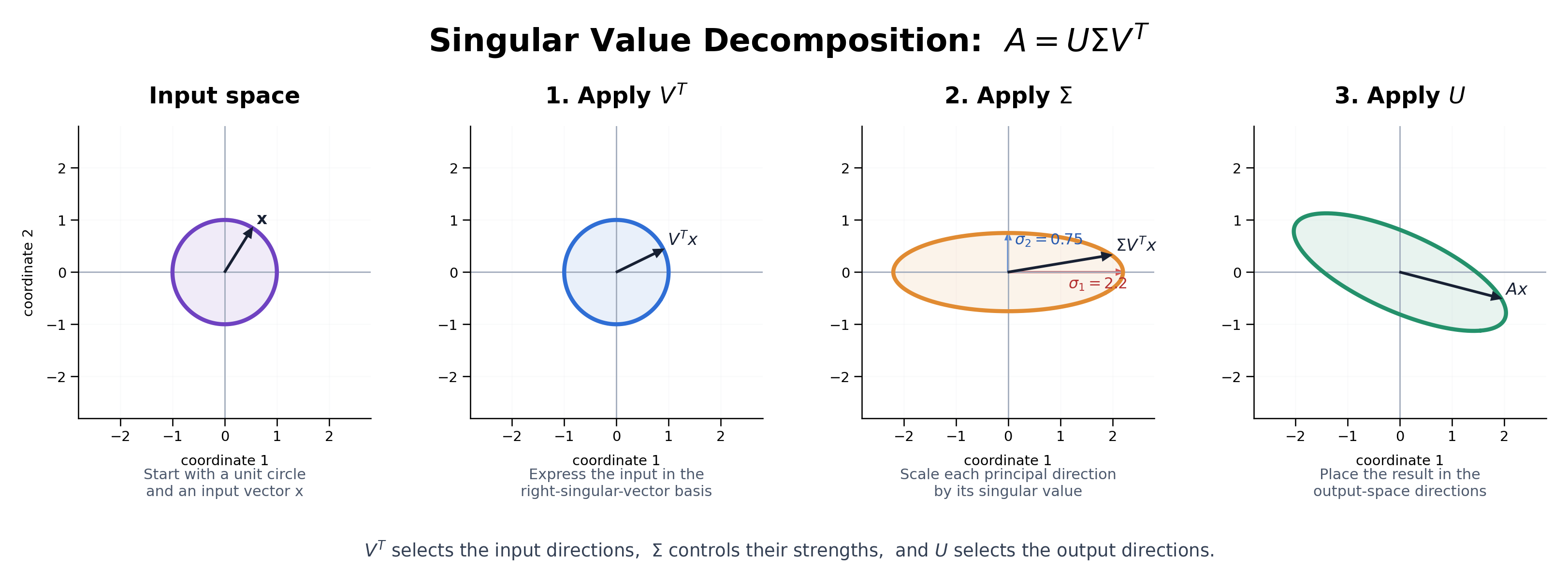
Singular Value Decomposition

• Diagonalization is generally defined for square matrices, while singular value decomposition can be applied to any rectangular or square matrix.

$$A=U\Sigma V^T$$

• For $A\in\mathbb{R}^{m\times n}$,

$$U\in\mathbb{R}^{m\times m}, \qquad \Sigma\in\mathbb{R}^{m\times n}, \qquad V\in\mathbb{R}^{n\times n}$$

• The columns of $V$ are the right singular vectors and represent orthonormal directions in the input space.
• The columns of $U$ are the left singular vectors and represent orthonormal directions in the output space.
• The diagonal entries of $\Sigma$ are the singular values.

$$\sigma_1\geq\sigma_2\geq\cdots\geq0$$

• For each singular-vector pair,

$$A\vec{v_i}=\sigma_i\vec{u_i}$$

• $\vec{v_i}$ is an input direction.

• $\sigma_i$ is the scaling factor.

• $\vec{u_i}$ is the corresponding output direction.

• The transformation $A$ can be interpreted as three steps:

  • $V^T$ expresses the input in the right singular-vector basis.
  • $\Sigma$ scales each direction by its singular value.
  • $U$ maps the scaled result into the output space.

• $U$ and $V$ are orthogonal matrices.

$$U^TU=\mathbb I, \qquad V^TV=\mathbb I$$

• The singular vectors and singular values are related to the eigenvectors and eigenvalues of $A^TA$ and $AA^T$.

$$A^TA\vec{v_i}=\sigma_i^2\vec{v_i}$$ $$AA^T\vec{u_i}=\sigma_i^2\vec{u_i}$$

• The rank of $A$ equals the number of nonzero singular values.
• SVD is commonly used for dimensionality reduction, data compression, noise reduction, pseudoinverses, and latent-factor analysis.

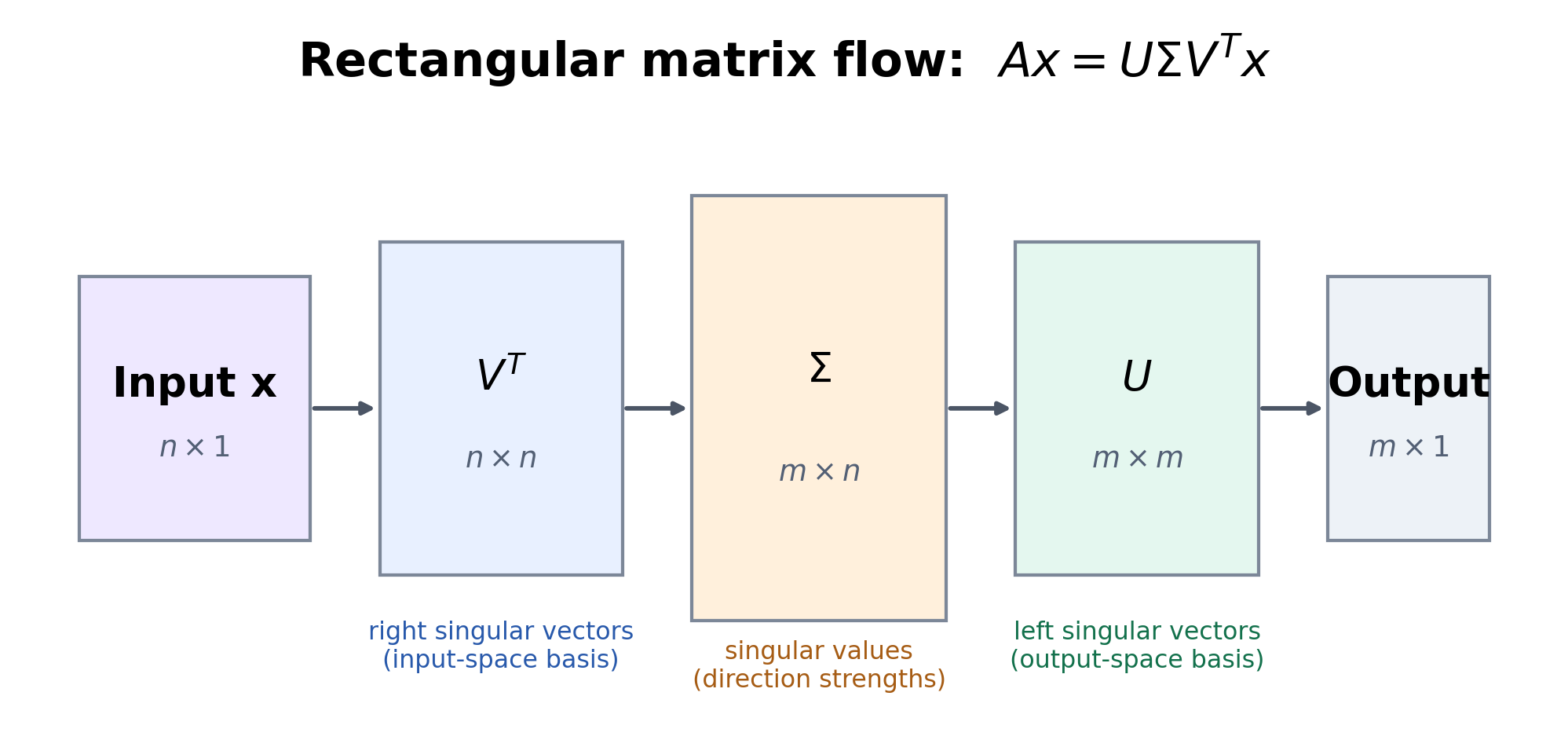
$$\underbrace{x}_{n\times 1} \xrightarrow{V^T} \underbrace{V^Tx}_{n\times 1} \xrightarrow{\Sigma} \underbrace{\Sigma V^Tx}_{m\times 1} \xrightarrow{U} \underbrace{U\Sigma V^Tx}_{m\times 1} = \underbrace{Ax}_{m\times 1}$$

• $U$ is such that the $m$ columns of $U$ are the eigenvectors of $AA^T$, known as the left singular vectors of $A$.
• $V$ is such that the $n$ columns of $V$ are the eigenvectors of $A^TA$, known as the right singular vectors of $A$.
• $\Sigma$ is a rectangular diagonal matrix with each element being the square root of an eigenvalue of $AA^T$ or $A^TA$.
• SVD allows us to construct a lower rank approximation of a rectangular matrix.
  • Choose only the top $r$ singular values in $\Sigma$.
  • The corresponding columns in $U$ and rows in $V^T$ are also selected.
• $V$ represents the principal directions in the input space, $U$ shows where those directions are mapped in the output space, and $\Sigma$ shows how much each direction is scaled.

Gradient

$$\nabla_A f(A) = \begin{bmatrix} \frac{\partial f}{\partial A_{11}} & \cdots & \frac{\partial f}{\partial A_{1n}} \\ \vdots & \ddots & \vdots \\ \frac{\partial f}{\partial A_{m1}} & \cdots & \frac{\partial f}{\partial A_{mn}} \end{bmatrix}$$

• The gradient with respect to $A$ is a matrix that shows how the function $f(A)$ changes with respect to each element of $A$.

$$\left(\nabla_A f(A)\right)_{ij} = \frac{\partial f(A)}{\partial A_{ij}}$$

• Each element of the gradient measures how sensitive $f(A)$ is to a small change in the corresponding element $A_{ij}$.

• If $f(x_1,x_2)=x_1^2+2x_2^2$ then the gradient is

$$\nabla f(x) = \begin{bmatrix} 2x_1 \\ 4x_2 \end{bmatrix}.$$

• The gradient points in the direction of the steepest increase of the function.
  • $\nabla f(x)$ is a direction of steepest increase.
  • $-\nabla f(x)$ is a direction of steepest decrease.
• The magnitude of the gradient indicates how steeply the function increases.
• To reduce the function value, optimization moves in the opposite direction of the gradient. This method is called gradient descent.

$$x_{\mathrm{new}} = x_{\mathrm{old}} - \eta\nabla f(x_{\mathrm{old}})$$

• $\eta$ is the learning rate, which controls the size of each update step.

Hessian

$$f:\mathbb{R}^n\to\mathbb{R}$$ $$H(x) = \nabla_x^2f(x) = \begin{bmatrix} \frac{\partial^2f}{\partial x_1^2} & \cdots & \frac{\partial^2f}{\partial x_1\partial x_n} \\ \vdots & \ddots & \vdots \\ \frac{\partial^2f}{\partial x_n\partial x_1} & \cdots & \frac{\partial^2f}{\partial x_n^2} \end{bmatrix}$$

• A Hessian matrix is a square matrix containing all second-order partial derivatives of a scalar-valued function.

• It describes the local curvature of the function.

• If the second-order partial derivatives are continuous, then the Hessian is symmetric.

• If

$$f(x_1,x_2)=x_1^2+2x_2^2,$$

then the gradient is

$$\nabla f(x) = \begin{bmatrix} \frac{\partial f}{\partial x_1} \\ \frac{\partial f}{\partial x_2} \end{bmatrix} = \begin{bmatrix} 2x_1 \\ 4x_2 \end{bmatrix}.$$

• The Hessian is obtained by differentiating each component of the gradient with respect to every input variable.

$$H(x) = \begin{bmatrix} \frac{\partial}{\partial x_1} \left(\frac{\partial f}{\partial x_1}\right) & \frac{\partial}{\partial x_2} \left(\frac{\partial f}{\partial x_1}\right) \\ \frac{\partial}{\partial x_1} \left(\frac{\partial f}{\partial x_2}\right) & \frac{\partial}{\partial x_2} \left(\frac{\partial f}{\partial x_2}\right) \end{bmatrix}$$ $$= \begin{bmatrix} \frac{\partial}{\partial x_1}(2x_1) & \frac{\partial}{\partial x_2}(2x_1) \\ \frac{\partial}{\partial x_1}(4x_2) & \frac{\partial}{\partial x_2}(4x_2) \end{bmatrix} = \begin{bmatrix} 2&0 \\ 0&4 \end{bmatrix}.$$

• At a stationary point where $\nabla f(x)=0$:

  • If $H(x)\succ0$, then the point is a strict local minimum.
  • If $H(x)\prec0$, then the point is a strict local maximum.
  • If $H(x)$ has both positive and negative eigenvalues, then the point is a saddle point.
  • If $H(x)$ is only positive semidefinite or negative semidefinite, the Hessian test may be inconclusive.

• If $H(x)\succeq0$ for every $x$, then $f$ is convex.

• If $H(x)\preceq0$ for every $x$, then $f$ is concave.

Differentiating a Linear Function

• For a constant vector $b\in\mathbb{R}^n$,

$$f(x)=b^Tx = \sum_{i=1}^{n}b_ix_i$$

• When differentiating with respect to $x_k$, every term except $b_kx_k$ is treated as a constant.

$$\frac{\partial f(x)}{\partial x_k} = b_k$$

• Collecting all partial derivatives gives

$$\nabla_x f(x) = \begin{bmatrix} b_1\\ b_2\\ \vdots\\ b_n \end{bmatrix} = b$$

• Therefore,

$$\nabla_x(b^Tx)=b$$

• Since $f(x)=b^Tx$ is linear, its gradient is constant and does not depend on $x$.

Differentiating a Quadratic Function

• For $f(x)=x^TAx$, where $A\in\mathbb{R}^{n\times n}$,

$$\nabla_x f(x) = (A+A^T)x$$

• The two terms appear because each variable can occur in both positions of the product $x_ix_j$.

• If $A$ is symmetric, then $A=A^T$, so

$$\boxed{ \nabla_x(x^TAx)=2Ax }$$

• The $l$-th component of the gradient is

$$\frac{\partial f(x)}{\partial x_l} = (2Ax)_l = 2\sum_{i=1}^{n}A_{li}x_i$$

• Differentiating the $l$-th gradient component with respect to $x_k$ gives the $(l,k)$-th entry of the Hessian.

$$H_{lk} = \frac{\partial}{\partial x_k} \left( \frac{\partial f(x)}{\partial x_l} \right) = \frac{\partial}{\partial x_k} \left( 2\sum_{i=1}^{n}A_{li}x_i \right) = 2A_{lk}$$

• Therefore,

$$\boxed{ \nabla_x^2(x^TAx)=2A }$$

• The gradient depends on $x$, while the Hessian is constant because $f(x)=x^TAx$ is a quadratic function.