CNN 005

Computer Vision

• Classification
• Classification with Localization
• Object Detection

-	ANN	CNN
Input	1D vector	3D tensor (height, width, channels)
Connections	Fully connected	Local connections (receptive fields)
Overfitting	Prone to overfitting	Less prone to overfitting

Convolutional Neural Networks (CNN)

1. Convolutional Layer (CONV)
2. Pooling Layer (POOL)
3. Fully Connected Layer (FC)

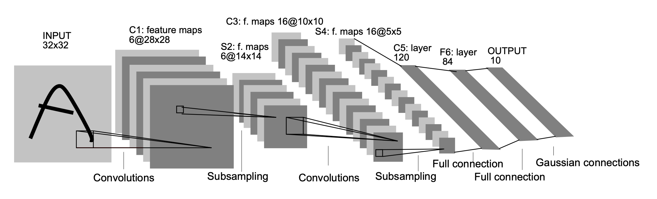
Convulutional Layer (CONV)

• The first layer to extraact features from an input image
• Core buildling block of a CNN
• Convolutions are basic operation in this layer
• A number of filters (e.g. edge detectors) are applied to the input image.

Padding

• Padding is used to control the spatial size of the output feature maps.
• Negative values at the edges can naturally arise because of padding, and they usually are not a big problem because activation functions and later layers come afterward.
• Input Matrix dimension: $n \times n \times c$ (height, width, channels)
• Filter size: $f \times f$
• Padding ($P$): 1, number of pixels added to the border of the input
• $(n \times n) * (f \times f) \to (n + 2P - f + 1) \times (n + 2P - f + 1)$
  • Example: $5 \times 5$ input with $3 \times 3$ filter and padding of 1 results in a $5 \times 5$ output feature map.
• if input and output matrix dimensions are the same, then $P = \frac{f - 1}{2}$.
• Valid padding ($P = 0$): No Padding
• Same padding ($P = \frac{f - 1}{2}$): Output size and input size is same, this requires appropriate padding.

Stride

• It is the number of pixels by which slide the filter across the input image.

No Padding Strides	Stride with Padding

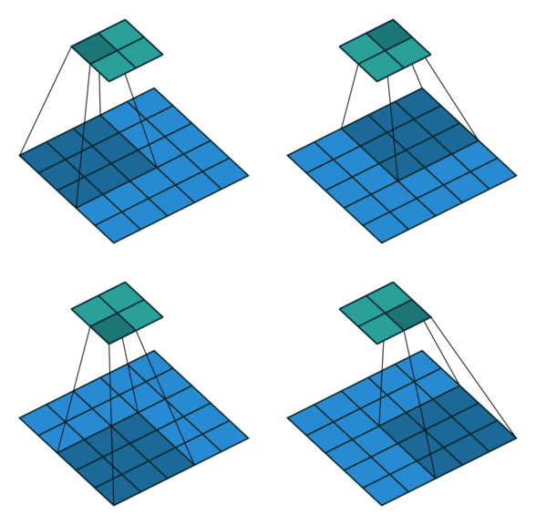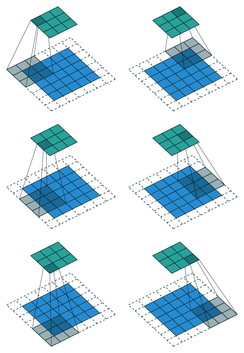• Github: vdumoulin/conv_arithmetic
• Input Matrix dimension: $n \times n$
• Filter size: $f \times f$
• Padding: $P$
• Stride: $S$
• Output Size = $\left\lfloor \frac{n + 2P - f}{S} + 1 \right\rfloor \times \left\lfloor \frac{n + 2P - f}{S} + 1 \right\rfloor$
  • Example: Input Matrix dimension: $5 \times 5$, Filter size: $3 \times 3$, Padding: $1$, Stride: $2$ results in an output size of $2 \times 2$.

Pooling Layer (POOL)

• Down sampling operation which reduces the dimensionality of a matrix.
• Reduces the number of parameters for large image, but retain the valuable information.
• Max pooling
• Average pooling
• Sum pooling

Fully Connected Layer (FC)

• a traditional Multi-layer Perception (MLP) layer
• For multi-class classification, usually Softmax activation is used.
• Softmax ensures the output.
• Output of the CONV and POOL layers represent a high level features of the Input image.
• The FC layer takes these features to classify the input image into the desired output classes.