CNN 004

Logistic Regression as Neural Network

• if $y = 1$
  • $L = -\log(\hat{y})$
  • if $\hat{y} \to 1$, then $L \to 0$ (low loss)
  • if $\hat{y} \to 0$, then $L \to \infty$ (high loss)
• if $y = 0$
  • $L = -\log(1 - \hat{y})$
  • if $\hat{y} \to 0$, then $L \to 0$ (low loss)
  • if $\hat{y} \to 1$, then $L \to \infty$ (high loss)

Gradient Descent

• it is an iterative approach for error correction in a machene learning model
• Find $w$ and $b$ that will minimize $GD(w, b)$ (requires Loss/Cost function)

1. Initialize $w$ and $b$
2. Perform Forward pass operation/calculations
3. Compute Loss/Cost function $L(a, y)$
4. Compute change in $w$ and $b$ (Take the partial derivative of the cost function with respect to Weights and bias $dw$ and $db$)
5. Update $w$ and $b$ ($w := w - \alpha dw$ and $b := b - \alpha db$)
6. Repeat from Step 2 with new values of $w$ and $b$ for 'n' number of iterations.

• $\alpha$ is the learning rate (hyperparameter) that controls how much we are adjusting the weights and bias of our model with respect to the loss gradient. It is a small positive value (e.g., 0.01, 0.001) that determines the step size at each iteration while moving toward a minimum of the loss function.

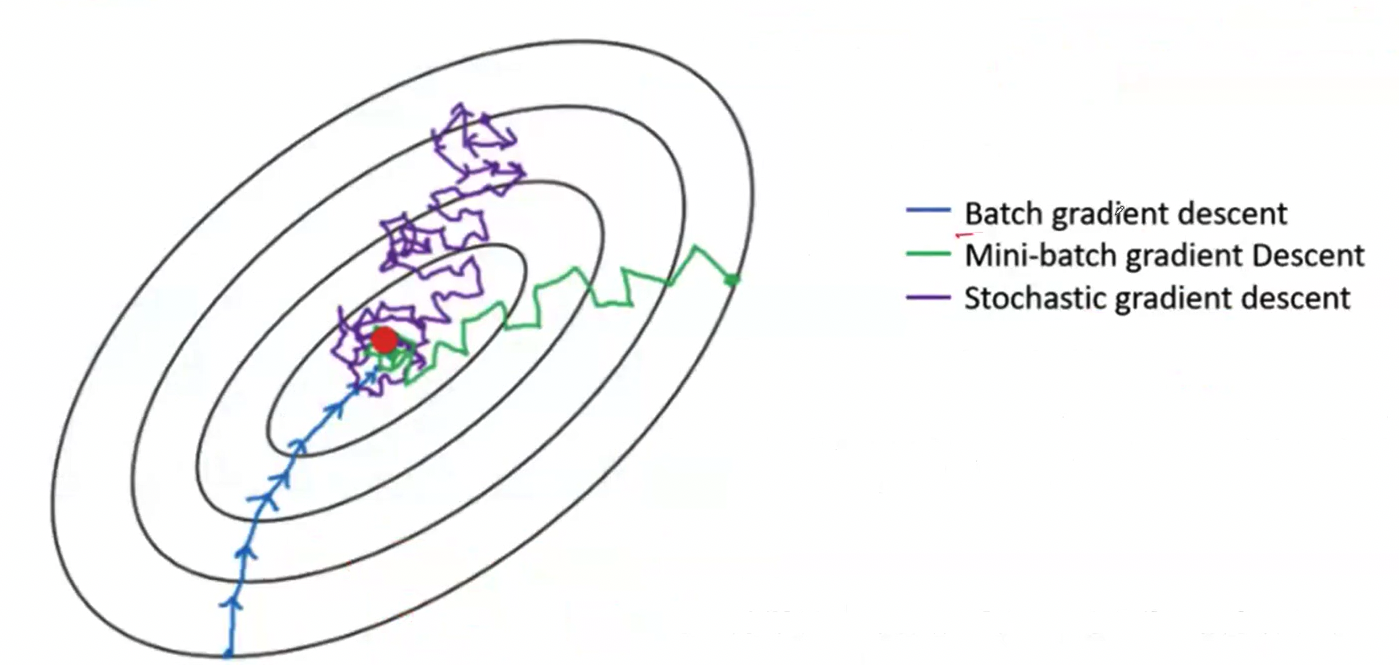
Gradient Descent Types

• Batch Gradient Descent (BGD)
• Stochastic Gradient Descent (SGD)
• Mini-batch Gradient Descent (MBGD)

Batch Gradient Descent (BGD)

1. Process each input sample and find the cost
2. Find the average cost oveer all input samples
3. Update $w$ and $b$ and repeat the steps for "n" epochs(iterations)

• Disadvantages:
  • It uses the complete dataset to calculate the gradients at every steps
  • Slow when training data is large
  • Difficult to find the learning rate
  • Difficult to ascertain the number of epochs(iterations)

Stochastic Gradient Descent (SGD)

Due to the random nature, the algorithm is much less regular than BGD.

1. Process a random input sample and find the cost.
2. Update $w$ and $b$, and repeat the steps for "n" iterations on the training samples.

• Advantages:
  • Computes gradient based on single input sample, which is memory efficient.
  • Much faster compared to BGD.
  • Possible to train on large datasets.
  • Randomness is helpful to escape local minima.
• Disadvantages:
  • Might not reach the optimal value, but very close to it.
    • Simulated annealing: Reduce the learning rate gradually
    • Create a Learning Schedule to determine the learning rate at each iteration.

Mini-batch Gradient Descent (MBGD)

1. Divide the tranining set into mini-batches of size $n$ (e.g., 64, 128, 256).
2. Process all the samples in a mini-batch and find the average cost
3. Update $w$ and $b$, and repeat the steps for "n" iterations/epoches on the traning samples.

• Advantages:
  • Computes gradient based on small sets of input smaple
  • Much faster compared to BGD.
  • Possible to train on large dataset.
  • Performance boost on matrix operations using GPUs.
  • Might not reach the optional value but, very close to it and possibly better than SGD.
• Disadvantages:
  • It may be harder to escape the local minima compared to SGD.

Exponentially Weighted Averages

• One of the popular algorithm for smoothing sequential data (time series data), aka. moving average.
• Weight the number of observations and using their average

$$V_0 = 0 \\ V_1 = 0.9 \cdot V_0 + 0.1 \cdot \theta_1 \\ V_2 = 0.9 \cdot V_1 + 0.1 \cdot \theta_2 \\ V_3 = 0.9 \cdot V_2 + 0.1 \cdot \theta_3 \\ \vdots \\ V_t = 0.9 \cdot V_{t-1} + 0.1 \cdot \theta_t \\ V_t = \beta \cdot V_{t-1} + (1 - \beta) \cdot \theta_t$$

$V_t$ is approximate average over $\approx \frac{1}{1 - \beta}$ time steps.

• For $\beta = 0.9$, $V_t$ is average over the last 10 time steps.
• For $\beta = 0.98$, $V_t$ is average over the last 50 time steps.
• For $\beta = 0.5$, $V_t$ is average over the last 2 time steps.

Optimizers

SGD with Moementum

At iteration $t$:

• Calculate $dw$ and $db$ on the current mini-batch (Hyper parameters: $\alpha$ and $\beta$)
• Update the velocity:
  • $V_{dw} = \beta V_{dw} + (1 - \beta) dw \rightarrow V_t = \beta V_{t-1} + (1 - \beta) \theta_t$
  • $V_{db} = \beta V_{db} + (1 - \beta) db$
• Update parameters:
  • $w := w - \alpha V_{dw}$
  • $b := b - \alpha V_{db}$

RMSProp

• Root Mean Square Propagation.
• Unpublished adaptive learning method by Geoffrey Hinton.
• Reduces oscillation but in a different way than Momentum.
• Divides the learning rate by an exponentially decaying average of squared gradients.
• Calculate $dw$ and $db$ on the current mini-batch
  • $S_{dw} = \beta S_{dw} + (1 - \beta) dw^2$
  • $S_{db} = \beta S_{db} + (1 - \beta) db^2$
• Update parameters:
  • $w := w - \alpha \frac{dw}{\sqrt{S_{dw}} + \epsilon}$
  • $b := b - \alpha \frac{db}{\sqrt{S_{db}} + \epsilon}$
  • $\epsilon$ is a small number to prevent division by zero (e.g., $10^{-8} \text{ to } 10^{-10}$)

Adam

• Adaptive Moment Estimation
• Combination of RMSProp and Momentum
• Work well for a wide range of non-convex optimization problems in machine learning.
• Calculate $dw$ and $db$ on the current mini-batch
  • $V_{dw} = \beta_1 V_{dw} + (1 - \beta_1) dw \leftarrow Momentum, \beta_1$
  • $V_{db} = \beta_1 V_{db} + (1 - \beta_1) db$
  • $S_{dw} = \beta_2 S_{dw} + (1 - \beta_2) dw^2 \leftarrow RMSProp, \beta_2$
  • $S_{db} = \beta_2 S_{db} + (1 - \beta_2) db^2$
• Update parameters:
  • $w := w - \alpha \frac{V_{dw}}{\sqrt{S_{dw}} + \epsilon}$
  • $b := b - \alpha \frac{V_{db}}{\sqrt{S_{db}} + \epsilon}$
  • $\epsilon$ is a small number to prevent division by zero (e.g., $10^{-8} \text{ to } 10^{-10}$)
• Hyper parameter guide:
  • $\alpha = 0.001$
  • $\beta_1 = 0.9$: Momentum term
  • $\beta_2 = 0.999$: Moving weighted average
  • $\epsilon = 10^{-8}$: To prevent division by zero
• ensmallen.org

Learning Rate Decay

• Speed-up the learning algorighm by slowing decreasing the learning rate $\alpha$ as the number of epochs increases.

Activation Functions

• Getting the output of a layer in a neural network and applying a non-linear function to it.
  • Sigmoid: $\sigma(x) = \frac{1}{1 + e^{-x}}$
  • Tanh: $\tanh(x) = \frac{2}{1 + e^{-2x}} - 1$
  • Used for binary classification in the output layer.
• ReLU: $A(x) = \max(0, x)$
  • Rectified Linear Unit
  • Avoids and rectifies vanishing gradient problem
  • Best used in hidden layers
  • Computationally less expensive than sigmoid and tanh
• Softmax: $S(x_i) = \frac{e^{x_i}}{\sum_{j} e^{x_j}}$
  • Turns numbers in probabilities that sum to 1.
  • Used for multi-class classification in the output layer.