IQC 005

Encoding

• Basis encoding: binary srings -> computational basis states
• Amplitude encoding: data values -> amplitudes of a quantum state
• Angle encoding: data values -> rotation angles on individual qubits

Basis Encoding

$x = b_1 b_2 ... b_n \rightarrow \ket{x} = \ket{b_1 b_2 ... b_n}$

• applying $X$ gates to flip qubits from $\ket{0}$ to $\ket{1}$ based on the binary representation of the data.
• $\ket{00} \rightarrow \ket{01}$ (X gate on the second qubit)
• $\ket{00} \rightarrow \ket{10}$ (X gate on the first qubit)
• Dataset superposition: to encode set $\{01, 11\}$
  • $\ket{S} = \frac{1}{\sqrt{2}}(\ket{01} + \ket{11})$
  • it requires Hadamard and/or controlled gates
• Hadamard transform
  • $\ket{H^{\otimes n}}\ket{0}^{\otimes n} = \frac{1}{\sqrt{2^n}} \sum_{x=0}^{2^n-1} \ket{x}$

import pennylane as qml

x = [int(b) for b in '1011']

def circuit(x):
  qml.BasisEmbedding(features=x, wires=range(len(x)))

dev = qml.device('default.qubit', wires=4)
qnode = qml.QNode(circuit, dev)

print(qml.draw(qml.transforms.decompose(qnode), show_all_wires=True)(x))

Amplitude Encoding

$x = [x_0, x_1, ..., x_{N-1}] \rightarrow |\psi\rangle = \sum_{i=0}^{2^N-1} x_k |k\rangle$

• The most qubit-efficient encoding method, since $n$ qubits can encode $2^n$ amplitudes.

$$\begin{align*} \ket{\bf 0} &\equiv \ket{000} \\ \ket{\bf 1} &\equiv \ket{001} \\ \ket{\bf 2} &\equiv \ket{010} \\ \ket{\bf 3} &\equiv \ket{011} \\ \ket{\bf 4} &\equiv \ket{100} \\ \ket{\bf 5} &\equiv \ket{101} \\ \ket{\bf 6} &\equiv \ket{110} \\ \ket{\bf 7} &\equiv \ket{111} \end{align*}$$

• The state can be rewritten more explicitly (for 3 qubits)

$\ket{\psi} = x_0 \ket{000} + x_1 \ket{001} + x_2 \ket{010} + x_3 \ket{011} + x_4 \ket{100} + x_5 \ket{101} + x_6 \ket{110} + x_7 \ket{111}$

• For $N$ data points, we need $n = \log_2(N)$ qubits.
• Converting to binary
  • with $n$ qubits, the computational basis states range from
    • $\ket{0}$ to $\ket{2^n - 1}$
  • $[x_0, x_1, ..., x_{N-1}]$ can be mapped to $x_0\ket{000} + x_1\ket{001} + \cdots + x_{N-1}\ket{(N-1)}$.
  • $b_i = \left\lfloor \frac{k}{2^i} \right\rfloor \bmod 2$.
• if $k = 5$
  • $b_0 = \left\lfloor \frac{5}{2^0} \right\rfloor \bmod 2 = 1$
  • $b_1 = \left\lfloor \frac{5}{2^1} \right\rfloor \bmod 2 = 0$
  • $b_2 = \left\lfloor \frac{5}{2^2} \right\rfloor \bmod 2 = 1$
  • gives $b_2 b_1 b_0 = 101$ (binary representation of 5)
  • $\ket{\bf 5} = \ket{101}$

Angle Encoding

• Each classical value controls the roation angle of a qubit gate.
• $x = [x_1, x_2, ..., x_n]$
• $RY(x_0) \ket{0} \otimes RY(x_1) \ket{0} \otimes ... \otimes RY(x_{n-1}) \ket{0}$
• where $RY(\theta) = \begin{bmatrix} \cos(\theta/2) & -\sin(\theta/2) \\ \sin(\theta/2) & \cos(\theta/2) \end{bmatrix}$ is the $Y$ rotation gate.

Summary of Encoding Methods

Method	Qubit cost	Eample Classical Data	Use Case	Circuit Complexity
Basis Encoding	1 qubit per bit	Binary strings ('1011')	Binary data, configs	Easy
Amplitude Encoding	$\log_2(N)$ qubits	Vector of real numbers	QML, optimization	Hard
Angle Encoding	1 qubit per data point	Vector of angles	Variational / hybrid algorithms	Easy

• Pennylane: BasisEmbedding, AmplitudeEmbedding, AngleEmbedding
• Qiskit: initialize
• PyTKET: StatePreparationBox

Amplitude Encoding Circuit

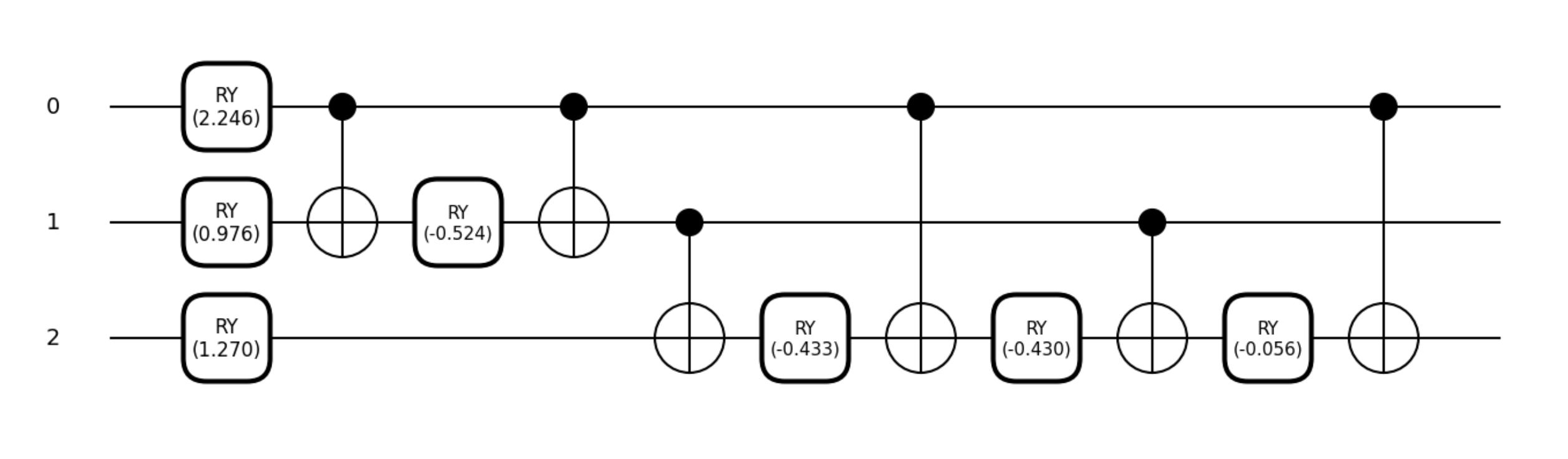
• The algorithm to prepare an arbitrary vector of length $2^n$ takes roughly that many gates. (e.g. $2^3 \approx 10$)

wires = [0, 1, 2]

def circuit(x):
  qml.AmplitudeEmbedding(x, wires)

dev = qml.device("default.qubit", wires=wires)
qnode = qml.QNode(circuit, dev)

# Random vector of length 8 (for 3 qubits)
x = np.random.rand(8)
# Normalize the vector to have unit length (required for quantum states)
x = x/np.sqrt(np.sum(x**2))

qml.draw_mpl(qnode)(x);
qml.draw_mpl(qml.transforms.decompose(qnode), decimals=3)(x);

from pytket.circuit import StatePreparationBox
from pytket.circuit.display import render_circuit_jupyter as draw

state_circ = pytket.circuit.Circuit(3)

# Example 3-qubit state to prepare
w_state = 1 / np.sqrt(3) * np.array([0, 1, 1, 0, 1, 0, 0, 0])

w_state_box = StatePreparationBox(w_state)
state_circ.add_gate(w_state_box, [0, 1, 2])

draw(state_circ)

pytket.transform.Transform.DecomposeBoxes().apply(state_circ)
draw(state_circ)

Different algorithms for Rotation gate

• Pennylane: Transformation of quantum states using uniformly controlled rotations $Ry(\theta) = e^{-\theta Y / 2} = \begin{bmatrix} \cos(\theta/2) & -\sin(\theta/2) \\ \sin(\theta/2) & \cos(\theta/2) \end{bmatrix}$

• PyTKET: Synthesis of Quantum Logic Circuits $R_y(\theta) = e^{-\theta \pi Y / 2} = \begin{bmatrix} \cos(\theta \pi / 2) & -\sin(\theta \pi / 2) \\ \sin(\theta \pi / 2) & \cos(\theta \pi / 2) \end{bmatrix}$

• Qiskit: Quantum Circuits for Isometries

• There are concreate algorithms for encoding classical data into quantum states, but this process is generally computationally expensive.

• It usually requires classical preprocessing, and the resulting circuit can be quite deep.

• In general, amplitude encoding an arbitary large vector is expensive.

• "a quantum computer can store an exponential amount of data" should be always considered together with the cost of state preparation.

• The real advantage of quantum computers does not appear for every problem, but only for specific problems that are well-suited to them.

  • Problems where state preparation is natural or efficient.
  • Problems that involve simulating quantum systems themselves.
  • Structured linear algebra, optimization, or sampling problems.
  • Problems where the input is already given as a quantum state.

Binary Logic Gates

a	b	sum	carry
0	0	0	0
0	1	1	0
1	0	1	0
1	1	0	1

• Sum $s = a \oplus b$ (XOR)
• Carry $c = a \cdot b$ (AND)

1. Declare registers
2. Apply opertions
3. Read the result

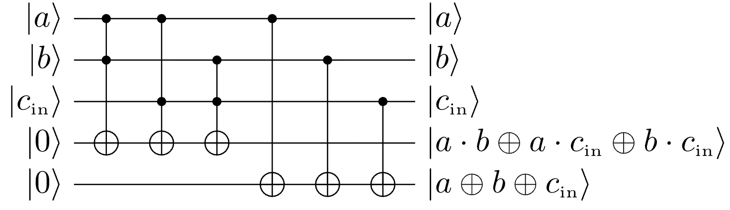
Full-Adder in Binary Logic

• Handles three inpus ($a$, $b$, and carry-in $c_{in}$) and produces two outputs (sum $s$ and carry-out $c_{out}$).

$a$	$b$	$c_{\text{in}}$	$s$	$c_{\text{out}}$
0	0	0	0	0
0	0	1	1	0
0	1	0	1	0
0	1	1	0	1
1	0	0	1	0
1	0	1	0	1
1	1	0	0	1
1	1	1	1	1

• $s = a \oplus b \oplus c_{in}$
• $c_{out} = (a \cdot b) \oplus (a \cdot c_{in}) \oplus (b \cdot c_{in})$
• A full-adder = two half-adders + an OR gate
• Chaning full-adders producs a ripple-carry adder for multi-bit numbers.

Quantum Arithmetic

• All quantum gates must be Unitary (Invertable)
• A classical half-adder discards input information after computing the sum and carry.
  • This irreversibility is forbidden in quantum circuits.
• The computation must be done in a way that preserves all input information.
  • XOR and AND operations must be implemented using reversible gates (e.g. Toffoli gate).
  • XOR $\rightarrow$ CNOT gate
  • AND $\rightarrow$ Toffoli gate

Classical op	Quantum gate
XOR $(a \oplus b)$	$\text{CNOT}(a, b) = \ket{a} \otimes \ket{b \oplus a}$
AND $(a \cdot b)$	$\text{CCX}\ket{a}\ket{b}\ket{c} = \ket{a} \ket{b} \ket{(a \cdot b) \oplus c}$

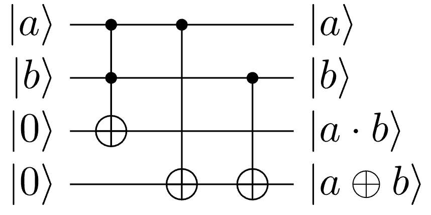
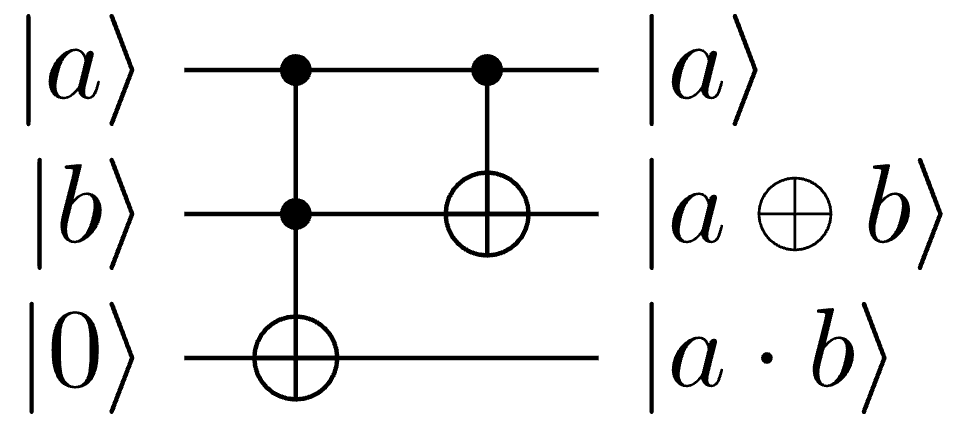
• With a third qubit initialized to $\ket{0}$, we can compute the AND of $a$ and $b$ without losing information about $a$ and $b$.

Half-Adder

Full-Adder

$C_{out} = (a \cdot b) \oplus (a \cdot c_{in}) \oplus (b \cdot c_{in})$ $s = a \oplus b \oplus c_{in}$

$CCX(a, b, c_{out}) \rightarrow CNOT(a, b) \rightarrow CCX(b, c_{in}, c_{out}) \rightarrow CNOT(b, c_{in})$

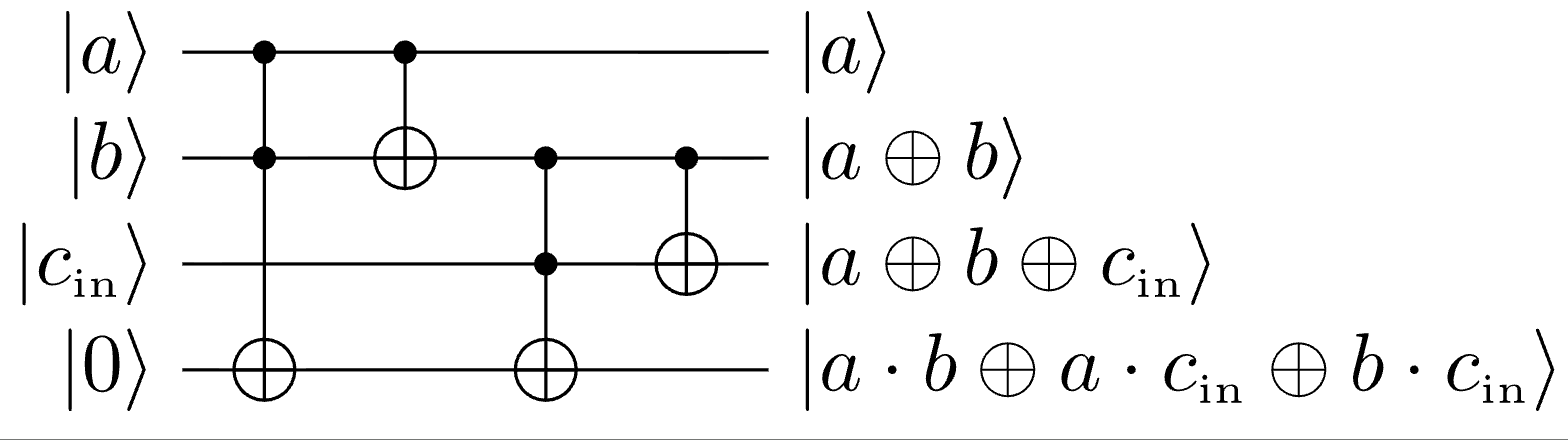
Ripple Carry Adder

• Two full-adder circuits in sequence, overlapping on the carry qubit ("rippling" the carry through the circuit).
• CDKM adder
  • Carry-out is the majority vote of the three inputs

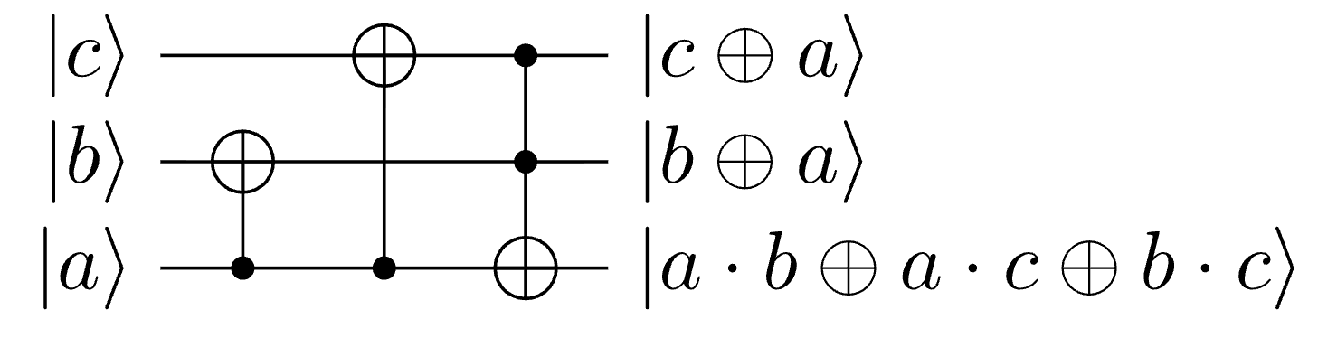
• MAJ: Majority, computes carry in-place using only 2 CNOTs + 1 Toffoli

  • $(c, b, a) \rightarrow (c \oplus a, b \oplus a, a \cdot b \oplus a \cdot c \oplus b \cdot c)$

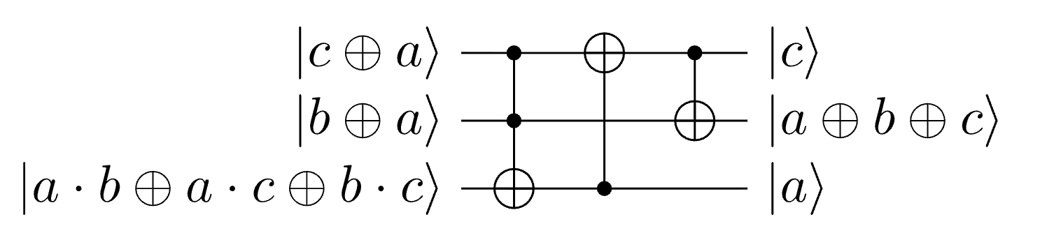
• UMA: UnMajority-and-Add, reverses MAJ but overwrites $b$ with the sum.

  • $c \oplus a, b \oplus a, c_{out} \rightarrow c, a\oplus b\oplus c, s$

• CDKM Ripple-Carry Adder: For two n-bit numbers, chain MAJ/UMA pairs, sharing the carry qubit.
  • CDKMRippleCarryAdder

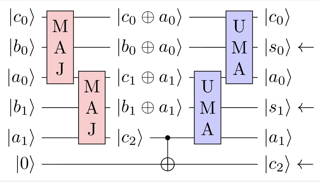
Quantum Multiplication

-	-	-	-	-	-	-
				1	1	0
x				1	0	1
				1	1	0
			0	0	0
+		1	1	0
		1	1	1	0	0

• Binary multiplication is "shift and add"
  • for each 1-bit in the multiplier, add a shifted version of the multiplicand to the result.
  • for each 0-bit, add nothing (or add a zero vector).
• In quantum, each partial addition is a conditional adder , every internal gate is controlled by a bit of the multiplier.

$CU = \ket{0}\bra{0} \otimes I + \ket{1}\bra{1} \otimes U$

Superposition

• Same adder circuit works on superposition of inputs

$\text{ADDER} \ket{2} (\ket{1} + \ket{3}) \ket{0} = \ket{2} (\ket{1} \ket{3})(\ket{3} \ket{5})$

• With one adder, both $2 + 1$ and $2 + 3$ are computed simultaneously.
• measurement collapses the superposition, we can only ever see one result per run. Either $2 + 1 = 3$ or $2 + 3 = 5$.
• Amplifying the probability of amplitudes corresponding to correct answers is a key part of quantum algorithms.

Summary

• Basis encoding maps each classical bit to a qubit, with 0 mapped to $|0\rangle$ and 1 mapped to $|1\rangle$.
• To encode 1011, we need X gates on qubits 0, 2, and 3 (assuming qubit 0 is the most significant bit).
• Applying an H gate (Hadamard gate) to each qubit puts the system in a uniform superposition over all basis states.
• Amplitude encoding of an arbitrary vector of size $2^n$ generally requires $O(2^n)$ gates.
• In angle encoding, each classical value $x_i$ becomes the rotation angle of an RY gate on the $i$-th qubit.
• Using the binary conversion formula, the decimal number 5 maps to $|101\rangle$ for 3 qubits.
• In short, in quantum addition, the sum is an XOR operation, and the carry is an AND operation.
• A quantum half-adder must keep the original inputs to remain reversible and maintain its unitary nature.
• The Toffoli gate is defined as: $|a\rangle|b\rangle|c\rangle \mapsto |a\rangle|b\rangle|c \oplus a \cdot b\rangle$.
• A full-adder should produce a carry-out as follows: $c_{\text{out}} = a \cdot b \oplus a \cdot c_{\text{in}} \oplus b \cdot c_{\text{in}}$.
• The following operation is reversible: $|a\rangle|b\rangle|c\rangle \mapsto |a\rangle|a \oplus b\rangle|c \oplus a \cdot b\rangle$.
• For addition "in superposition," measuring the output register yields exactly one of the partial sums, chosen probabilistically.
• The MAJ circuit computes the majority function as: $a \cdot b \oplus a \cdot c \oplus b \cdot c$.
• The QASM snippet for a half-adder uses ccx q[0], q[1], q[2] to compute the carry ($a \cdot b$) and a cx q[0], q[1] (or cx q[1], q[0]) gate to compute the sum ($a \oplus b$).
• Quantum multiplication can be implemented via conditional addition, one per multiplier bit.