OpenQASM

OpenQASM 2.0

오픈캐즘

OPENQASM 2.0; // 언어 버전 선언

qreg q[1]; // 큐비트 레지스터 q를 선언 (큐비트 1개, 초기 상태 |0⟩)
creg c[1]; // 고전 비트 레지스터 c를 선언 (측정 결과 저장용)

h q[0]; // Hadamard 게이트 적용: |0⟩ → (|0⟩ + |1⟩) / √2

measure q[0] -> c[0]; // q[0]을 측정하고 결과(0 또는 1)를 c[0]에 저장

OPENQASM 2.0;

qreg q[10]; // ∣0000000000⟩
creg c[10];

// x 게이트를 사용하여 처음 세 큐비트를 ∣1⟩ 상태로 변경
x q[0]; ∣1000000000⟩
x q[1]; ∣1100000000⟩
x q[2]; ∣1110000000⟩

measure q[0] -> c[0]; // 1
measure q[1] -> c[1]; // 1
measure q[2] -> c[2]; // 1

Linear Algebra

Vectors

• In quantum computing, vectors represent quantum states.
• A 2-dimensional vactor can be written as:
• $|\psi\rangle = \begin{pmatrix} \psi_0 \\ \psi_1 \end{pmatrix}$

Computational Basis

$|0\rangle = \begin{pmatrix} 1 \\ 0 \end{pmatrix}, \quad |1\rangle = \begin{pmatrix} 0 \\ 1 \end{pmatrix}$

• $|\psi\rangle$ is a linear combination of basis states as follows:
• $|\psi\rangle = \psi_0|0\rangle + \psi_1|1\rangle = \begin{pmatrix} \psi_0 \\ \psi_1 \end{pmatrix}$

Indentity Matrix

• $\mathbb I \psi\rangle = \begin{bmatrix} \psi_0 \\ \psi_1 \end{bmatrix}$
• $\mathbb I^2 = \begin{bmatrix} 1 & 0 \\ 0 & 1 \end{bmatrix}$

Conjugate Transpose

• Bra: $|\psi\rangle^\dagger = \begin{pmatrix} \psi_0 \\ \psi_1 \end{pmatrix}^\dagger = \begin{pmatrix} \overline{\psi_0} & \overline{\psi_1} \end{pmatrix} = \langle \psi|$
  • $\langle \psi| := |\psi\rangle^\dagger$
  • ket: $|\psi\rangle$
  • bra: $\langle \psi|$
  • bra + ket: dot product $\langle \phi|\psi\rangle$
• Dagger: $A = \begin{bmatrix} a & b \\ c & d \end{bmatrix} \implies A^\dagger = \begin{bmatrix} \overline{a} & \overline{c} \\ \overline{b} & \overline{d} \end{bmatrix}$

psi_dagger = psi.conjugate().T
psi_dagger = psi.conjugate().transpose()
psi_dagger = psi.H

• $(\alpha A)\dagger = \overline\alpha A^\dagger$
• $(A^\dagger)^\dagger = A$
• $(A + B)^\dagger = A^\dagger + B^\dagger$
• $(AB)^\dagger = B^\dagger A^\dagger$

Hermitian

• A matrix is equal to its conjugate transpose.
• $H = H^\dagger$

A_dagger = A.H
AA_dagger = A * A_dagger
# (AA†)†=AA†?
is_hermitian = AA_dagger.is_hermitian

Unitary

• A matrix whose conjugate transpose is also its inverse.
• $U^\dagger U = U U^\dagger = \mathbb I$
• $U = \begin{pmatrix} \cos\theta & \sin\theta \\ -\sin\theta & \cos\theta \end{pmatrix}$

U = Matrix([
  [cos(theta), sin(theta)], 
  [-sin(theta), cos(theta)]
])

U_dagger = U.H
U_dagger_U = trigsimp(U_dagger * U)

is_unitary = U_dagger_U == I

Inner Product

• $\langle \psi|\phi\rangle = \begin{pmatrix} \overline{\psi_0} & \overline{\psi_1} \end{pmatrix} \begin{pmatrix} \phi_0 \\ \phi_1 \end{pmatrix} = \overline{\psi_0}\phi_0 + \overline{\psi_1}\phi_1$
• $|\langle \psi|\phi\rangle|^2 = \langle \psi|\phi\rangle \langle \phi|\psi\rangle$
• $|\langle\psi|\phi\rangle| = |\langle\phi|\psi\rangle|$

Orthogonality

• $|0\rangle = \begin{pmatrix} 1 \\ 0 \end{pmatrix}, \quad |1\rangle = \begin{pmatrix} 0 \\ 1 \end{pmatrix}$
  • orthonormal basis
• $\langle 0 | 1 \rangle = \begin{pmatrix} 1 & 0 \end{pmatrix} \begin{pmatrix} 0 \\ 1 \end{pmatrix} = 0$
  • $\langle 1 | 0 \rangle = 0$
• $\langle 0 | 0 \rangle = \begin{pmatrix} 1 & 0 \end{pmatrix} \begin{pmatrix} 1 \\ 0 \end{pmatrix} = 1$
  • $\langle 1 | 1 \rangle = 1$

$\langle \psi|\phi\rangle = \overline{\psi_0}\phi_0 + \overline{\psi_1}\phi_1$

• $|\psi\rangle = \psi_0|0\rangle + \psi_1|1\rangle, \quad |\phi\rangle = \phi_0|0\rangle + \phi_1|1\rangle$
• $\langle \psi| = \overline{\psi_0}\langle 0| + \overline{\psi_1}\langle 1|$
• $\langle \psi|\phi\rangle = \overline{\psi_0}\phi_0\langle 0|0\rangle + \overline{\psi_0}\phi_1\langle 0|1\rangle + \overline{\psi_1}\phi_0\langle 1|0\rangle + \overline{\psi_1}\phi_1\langle 1|1\rangle$
• $\langle 0|1\rangle = 0, \quad \langle 1|0\rangle = 0$

Magnitude

$\|\psi\rangle\|^2 = |\psi_0|^2 + |\psi_1|^2$

• $\|\psi\rangle\| = \sqrt{\langle \psi|\psi\rangle} = \sqrt{|\psi_0|^2 + |\psi_1|^2}$
• $\| |\psi\rangle\|^2 = \langle \psi|\psi\rangle$
  • $\langle \psi|\psi\rangle = \overline{\psi_0}\psi_0 + \overline{\psi_1}\psi_1 = |\psi_0|^2 + |\psi_1|^2$

Outer product

• $|\psi\rangle\langle\phi| = (\psi_0 | 0\rangle + \psi_1 |1\rangle)(\overline{\phi_0}\langle 0| + \overline{\phi_1}\langle 1|) \\ \quad =\psi_0\overline{\phi_0}|0\rangle\langle 0| + \psi_0\overline{\phi_1}|0\rangle\langle 1| + \psi_1\overline{\phi_0}|1\rangle\langle 0| + \psi_1\overline{\phi_1}|1\rangle\langle 1|$
• $|\psi\rangle\langle\phi| = \begin{pmatrix} \psi_0 \\ \psi_1 \end{pmatrix} \begin{pmatrix} \overline{\phi_0} & \overline{\phi_1} \end{pmatrix} = \begin{pmatrix} \psi_0\overline{\phi_0} & \psi_0\overline{\phi_1} \\ \psi_1\overline{\phi_0} & \psi_1\overline{\phi_1} \end{pmatrix}$
• $|0\rangle = \begin{pmatrix} 1 \\ 0 \end{pmatrix}, \quad |1\rangle = \begin{pmatrix} 0 & 1 \end{pmatrix}$
• $|0\rangle\langle 0| = \begin{pmatrix} 1 \\ 0 \end{pmatrix} \begin{pmatrix} 0 & 1 \end{pmatrix} = \begin{pmatrix} 0 & 1 \\ 0 & 0 \end{pmatrix}$
• $A = \begin{pmatrix} a_{00} & a_{0 1} \\ a_{1 0} & a_{1 1} \end{pmatrix} \\ \quad = a_{00}|0\rangle\langle 0| + a_{01}|0\rangle\langle 1| + a_{10}|1\rangle\langle 0| + a_{11}|1\rangle\langle 1|$

Tensor Product

• $|\psi\rangle \otimes |\phi\rangle = \begin{pmatrix} \psi_0 \\ \psi_1 \end{pmatrix} \otimes \begin{pmatrix} \phi_0 \\ \phi_1 \end{pmatrix} = \begin{pmatrix} \psi_0\phi_0 \\ \psi_0\phi_1 \\ \psi_1\phi_0 \\ \psi_1\phi_1 \end{pmatrix}$
• $|\psi\rangle \otimes |\phi\rangle \equiv |\psi\rangle|\phi\rangle \equiv |\psi\phi\rangle$
• $A \otimes B = \begin{pmatrix} a_{00}B & a_{01}B \\ a_{10}B & a_{11}B \end{pmatrix}$
• $|0\rangle \langle 1| \otimes |1\rangle \langle 0| = \begin{pmatrix} 0 & 1 \\ 0 & 0 \end{pmatrix} \otimes \begin{pmatrix} 0 & 0 \\ 1 & 0 \end{pmatrix}$
• $|0\rangle \langle 1| \otimes |1\rangle \langle 0| = \begin{pmatrix} 0\begin{pmatrix} 0 & 0 \\ 1 & 0 \end{pmatrix} & 1\begin{pmatrix} 0 & 0 \\ 1 & 0 \end{pmatrix} \\ 0\begin{pmatrix} 0 & 0 \\ 1 & 0 \end{pmatrix} & 0\begin{pmatrix} 0 & 0 \\ 1 & 0 \end{pmatrix} \end{pmatrix} = \begin{pmatrix} 0 & 0 & 0 & 0 \\ 0 & 0 & 1 & 0 \\ 0 & 0 & 0 & 0 \\ 0 & 0 & 0 & 0 \end{pmatrix}$
• $|0\rangle \langle 1| \otimes |1\rangle \langle 0| \equiv (|0\rangle \otimes |1\rangle)(\langle 1| \otimes \langle 0|) \\ \quad \equiv |0\rangle|1\rangle \langle 0|\langle 1| \\ \quad \equiv |01\rangle \langle 10|$
  • $ket \otimes ket, \quad bra \otimes bra$

Qubit

$|\psi\rangle = \alpha|0\rangle + \beta|1\rangle$

• where $\alpha, \beta$ are complex numbers satisfying $|\alpha|^2 + |\beta|^2 = 1$.
• phase factor: $e^{i\phi}$, turn the state by angle $\phi$ in the complex plane, but does not affect measurement probabilities.
  • $|e^{i\phi}| = 1$

One-Qubit Gates

Identity Gate

$\mathbb{I} = \begin{pmatrix} 1 & 0 \\ 0 & 1 \end{pmatrix}$

Pauli-X Gate

$X = \begin{pmatrix} 0 & 1 \\ 1 & 0 \end{pmatrix}$

• NOT gate

Pauli-Y Gate

$Y = \begin{pmatrix} 0 & -i \\ i & 0 \end{pmatrix}$

Pauli-Z Gate

$Z = \begin{pmatrix} 1 & 0 \\ 0 & -1 \end{pmatrix}$

Hadamard Gate

$H = \frac{1}{\sqrt{2}} \begin{pmatrix} 1 & 1 \\ 1 & -1 \end{pmatrix}$

Rotation Gate

$R(\theta) = \begin{pmatrix} \cos{\theta} & \sin{\theta} \\ -\sin{\theta} & \cos{\theta} \end{pmatrix}$

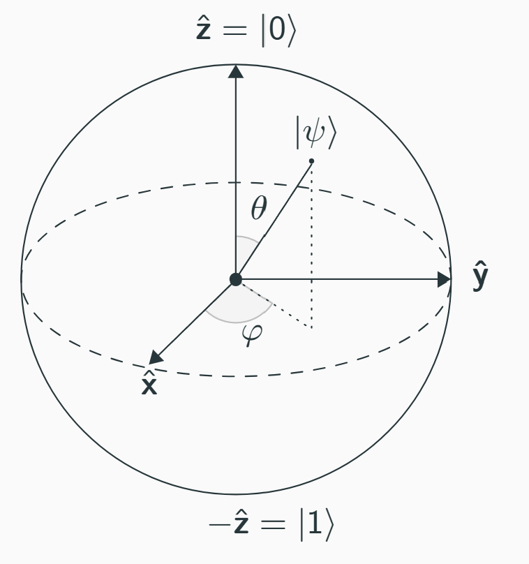
The Bloch Sphere

$|\psi\rangle = \cos(\theta) |0\rangle + e^{i\phi}\sin(\theta)|1\rangle$

• where $0 \leq \theta \leq \pi$ and $0 \leq \phi < 2\pi$.
• $\theta$: the polar (or colatitude) angle, measured from the "north pole" of the sphere.
  • polar angle: 편각
• $\phi$: the azimuthal (or longitude) angle around the equator.
  • azimuthal angle: 방위각

Two-Qubit Gates

CNOT Gate

Controlled-NOT or CX gate

$CNOT = \begin{pmatrix} 1 & 0 & 0 & 0 \\ 0 & 1 & 0 & 0 \\ 0 & 0 & 0 & 1 \\ 0 & 0 & 1 & 0 \end{pmatrix}$

• CNOT gate flips the second qubit (target) if the first qubit (control) is $|1\rangle$.

SWAP Gate

$SWAP = \begin{pmatrix} 1 & 0 & 0 & 0 \\ 0 & 0 & 1 & 0 \\ 0 & 1 & 0 & 0 \\ 0 & 0 & 0 & 1 \end{pmatrix}$

• SWAP gate exchanges the states of the two qubits.

Controlled-Z Gate

$CZ = \begin{pmatrix} 1 & 0 & 0 & 0 \\ 0 & 1 & 0 & 0 \\ 0 & 0 & 1 & 0 \\ 0 & 0 & 0 & -1 \end{pmatrix}$

• CZ gate applies a Z gate to the second qubit if the first qubit is in state $|1\rangle$.

Bases

• Computational Basis: $\{|0\rangle, |1\rangle\}$
• two qubits: $\{|00\rangle, |01\rangle, |10\rangle, |11\rangle\}$
• three qubits: $\{|000\rangle, |001\rangle, |010\rangle, |011\rangle, |100\rangle, |101\rangle, |110\rangle, |111\rangle\}$

Rule of Thumb

What starts on the left of the tensor product stays on the left.

• $|\psi\rangle \otimes |\phi\rangle \equiv |\psi\rangle|\phi\rangle \equiv |\psi\phi\rangle$
• $(|\psi\rangle \otimes |\phi\rangle)^* = \langle\psi| \otimes \langle\phi|$
• $(\alpha |\psi\rangle + \beta |\phi\rangle) \otimes |\omega\rangle = \alpha|\psi\rangle \otimes |\omega\rangle + \beta |\phi\rangle \otimes | \omega\rangle$
• $(\langle\psi| \otimes \langle\phi|)(|\omega\rangle \otimes |\eta\rangle) = \langle\psi|\omega\rangle \cdot \langle\phi|\eta\rangle)$
• $(A + B) \otimes C = A \otimes C + B \otimes C$
• $A \otimes (B + C) = A \otimes B + A \otimes C$
• $(A \otimes B)(C \otimes D) = (AC) \otimes (BD)$
• $(A \otimes B)^* = A^* \otimes B^*$

Entanglement

• $|\Psi\rangle = \alpha_{00} |00\rangle + \alpha_{01} |01\rangle + \alpha_{10} |10\rangle + \alpha_{11} |11\rangle$
  • where $\|\Psi\rangle\|^2 = 1$
• If the state is not separable, it is entangled.
• A state is separable if it can be written as a tensor product of two individual qubit state.
• $|\Psi\rangle = \frac{1}{\sqrt{2}} (|00\rangle + |01\rangle) \\ \quad = \frac{1}{\sqrt{2}} |0\rangle \otimes (|0\rangle + |1\rangle) \\ \quad = |0\rangle \otimes \frac{1}{\sqrt{2}} (|0\rangle + |1\rangle)$
  • separable
• $|\Phi\rangle = \frac{1}{\sqrt{2}} (|00\rangle + |11\rangle)$
  • $|\Phi\rangle = (a|0\rangle + b|1\rangle) \otimes (c|0\rangle + d|1\rangle) \\ \quad = ac|00\rangle + ad|01\rangle + bc|10\rangle + bd|11\rangle$
  • $ad = 0, \quad bc = 0$ which is impossible.
  • entangled

Latex

• \texttip{}: Displays a tooltip when hovering over the equation.
• \toggle{}: Toggles between two expressions.
• \begin{align}: Aligns equations, where the ampersand (&) marks the alignment points.
• \bbox[color, padding]{}: Puts a bounding box with the specified color and padding around an expression.
• \boldsymbol{}: Renders a bold version of symbols like variables.
• \cancel{}: Strikes through an expression.
• \cancelto{value}{}: Strikes through and labels with the specified value.
• \begin{cases}: Creates a piecewise function with conditions.
• \color{}: Applies a color to text or math expressions. You can use predefined colors or hex values.
• \enclose{}: Encloses an expression with various effects like circles or strikes.
• [mathcolor="color", mathbackground="color"]: Adds custom colors to the enclosing effect.
• \xmapsto{}: Creates an arrow with a label for mapping.
• \xlongequal{}: Creates a long equals sign with a label.
• \ce{}: Renders chemical equations or formulas.
• \newcommand{\ket}[1]{\left|#1\right\rangle}: defines a custom command for ket notation. \ket{\psi}
• \tag{}: Assigns a custom tag to an equation.
• \unicode{}: Inserts a Unicode character using its code.

Ref

• OpenQASM 2.0