IAI +007
· 8 min read

Computer vision
- a field of artificial intelligence enabling computers and systems to derive meaningful information from digital images, videos and other visual inputs.
- vision is a perceptual channel that accepts a stimulus and reports soome representation of the world
- computer vision enables intelligent agents to see, observe and understand of environment
Core problems of CV
- reconstruction: an agent builds a mode lfo the world from an image or a set of images
- recognition: an agent draws distinctions amont the objects it encounters based on visual and other information.
- image classification
- object detection
- image segmentation
Classic approaches to object recognition problems
- feature-based object recognition approach
- works well for faces looking directly at the camera.
- pattern-element-based object recognition approach
- a useful abstraction is to assume that some objects are made up of local patterns which tend to move around with respect to one another.
- we can model objects with pattern elements.
Modern approaches to object recognition problems
- deep learning networks
- to recognition problems enables that features can be automatically learned and extracted from raw image data compares with the manual feature extraction in the classic approaches.
- AlexNet, VGGNet, GoogleNet, ResNet, DenseNet, EfficientNet, RegNet...
- basic models and derived models
- YOLO, SSD, RetinaNet, R-CNN...
Evaluation metrics for image classification
| Metric | Definition | Use case |
|---|---|---|
| Accuracy | the percentage of correcly predicted labels out of all predictions made | commonly used in balanced datasets but can be mis leading in imbalanced classes |
| Precisino | the ratio of correctly predicted positive observations to the total predicted positives. | useful when the cost of false positives is high (e.g., spam detection) |
| Recall (Sensitivity or True Positive Rate) | the ratio of correctly predictted observations to all the actual positives | important when the cost of false negatives s high (e.g., disease detection) |
| F1 Score | the harmonic mean of Precision and Recall | used when you need to balance precision and recall, especially in imbalanced datasets |
| Specificity (True Negative Rate) | the ratio of correctly predicted negative observations to all the actual negatives. | important when false positives should be minimized (e.g. medical tests for diseases) |
| Confusion Matrix | a table used to describe the performance of a classification model by showing the true positive, false positive, true negative, and false negative counts | provides a comprehensive understanding of a models' performance across all classes |
| ROC Curve (Receiver Operation Characteristic) | a graphical representation of the classifier's performance across all thresholds, plotting the true positive rate (recall) against the false positive rate (1 - specificity) | used to evaludate binary classirifres and compare models |
| AUC (Area Under the Curve) | the area under the ROC curve, providing a single number summary of the models' ability to discriminate between positive and negative classes | useful for evaluating binary classification models, particularly when dealing with imbalanced datasets. |
Confusion Matrix
| Actual class ➡️ Predicted class ⬇️ | Positive | Negative | Metric |
|---|---|---|---|
| Positive | TP: True Positive | FP: False Positive | Precision: |
| Negative | FN: False Negative | TN: True Negative | Negative Predictive Value: |
| Metric | Recall or Sensitivity: | Specificity: | Accuracy: |
ROC Curve
- Sort predicted probabilities
- Try multiple thresholds
- For each threshold, compute predicted labels
- Compute TPR and FPR
- Plot ROC curve (FPR vs TPR) i. ii.
- Compute AUC as area under ROC curve
from sklearn.metrics import roc_curve, roc_auc_score
fpr, tpr, thresholds = roc_curve(y_true, y_scores)
auc = roc_auc_score(y_true, y_scores)
Evaluation metric for object detection
| Metric | Definition | Use case |
|---|---|---|
| Intersection over Union (IoU) | measures how much the predicted bounding box overlaps with the ground truth. | |
| Precision | the ratio of correctly predicted postive observations to the total predicted positives | |
| Recall | the ratio of correctly predicted observations to all the actual positives | |
| F1 Score | the harmonic mean of Precision and Recall | |
| Average Precision (AP) | Precision-Recall Curve: Precision vs Recall at different thresholds AP: Area under the Precision-Recall curve (per class) | |
| Mean Average Precision (mAP) | mean of AP across all classes | provides a comprehensive understanding of a models' performance across all classes |
| AP@[.50:.95] | COCO benchmark | Averages AP at IoU threshold from 0.5 to 0.95 in steps of 0.05 |
- AP is computed by summing trapezoid areas under the Precision-Recall curve.
Convolutional Neural Network (CNN)
- contains spatially local connectinos at lest in the early layers
- has patterns of weights that are replicated across the units in each layer.
- use a kernel to detect patterns of weights that is replicated across multiple local regions in an image
- use convolution that applies the kernel to the pixels of the image
Input
   ↓
[Conv → ReLU] → [Pooling]
   ↓
[Conv → ReLU] → [Pooling]
   ↓
Flatten (2D → 1D 벡터)
   ↓
Fully Connected Layer
   ↓
Output Layer (Softmax/Sigmoid)
- : the -th output element (convolution result)
- : index inside the kernel (from 1 to )
- : kernel size (number of elements in the kernel)
- : the -th kernel weight (filter element)
- : input sequence (the original data)
- : the input element aligned with kernel position when shifted by stride
- : stride (step size of the kernel movement)
- : total shift in the input for the -th convolution
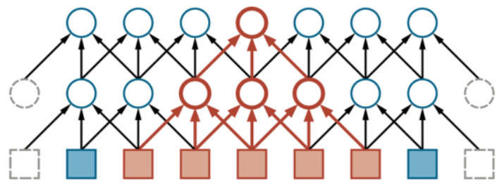
Receptive Field
- the receptive field of a neuron is the portion of the sensory input that can affect aht neuron's activation.
- In CNNs, the receptive field of a unit in the first hidden layer is small.
- just the size of the kernel, e.g., 3x3 or 5x5.
- In the deeper layers of the network, it can be much larger.
- : receptive field size at the layer
- : kernel size at the layer
- : stride at the layer
| Layer | Kernel k | Stride s | Calculation | Result RF |
|---|---|---|---|---|
| Conv1 | 3 | 1 | 1 + (3-1)*1 | 3 |
| Pool1 | 2 | 2 | 3 + (2-1)*1 | 4 |
| Conv2 | 3 | 1 | 4 + (3-1)*2 | 8 |
Pooling
- works like a convolutional layer, with a kernel size and stride , but the operation is applied is fixed rather than learned.
- no activation fucntion is associated with the pooling layer.
- common forms of pooling
- average pooling
- max pooling: saying a feature exists somewhere in the unit's receptive field.
Dropout
- a way to reduce the test-set error of a network to increase its ability of generalization.
- makes a etwork herder to fit the traninig set.
- the network is created by deactivating a randomly chosen subset of the units (dropout rate).
- cannot explain why it works but the results is better
Batch Normalization
- modern neural networks are almost always trained with some variant of stochastic gradient descent (SGD).
- Batch normlization rescales the values generated at the internal layers of the network from the examples within each minibatch.
- it standardizes the input to a layer for each mini-batch.
- standardizes the mean and variance of the values.
- maeks it much simpler to train a deep network.
Tranining in a CNN
- Forward pass
- Backward pass
- Parameter update
Variants of CNNs
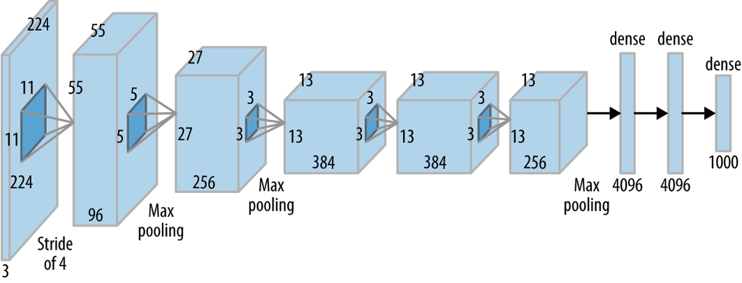
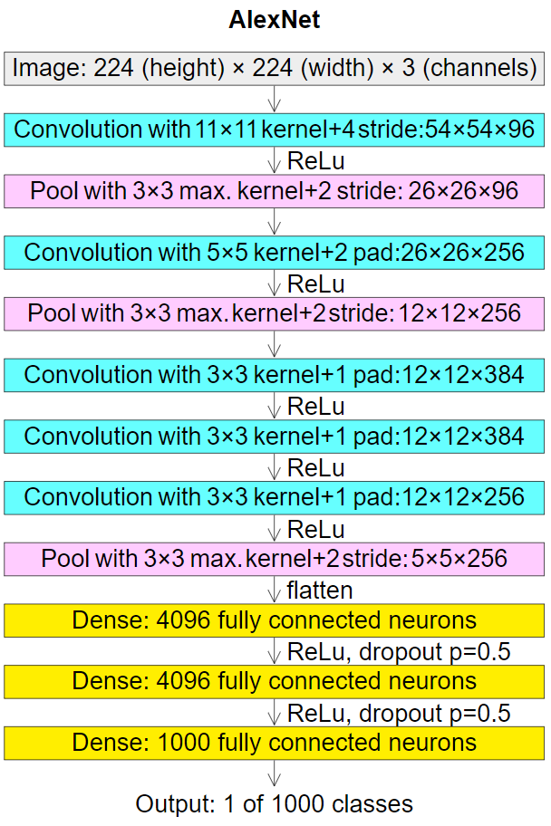
AlexNet
ResNet
- stands for a residual neural network.
- was designed to enable hundreds or thousands of convolutional layers.
- Residual neural networks do this by utilizing skip connections, or shortcurts to jump over some layers.
- was an innovative solution to the "vanishing gradient" problem.
x ────────────────► (+) ──► y
   │                     ▲
   ▼                     │
 [Conv → ReLU → Conv] = F(x)
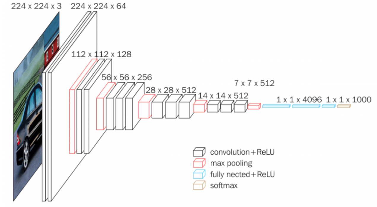
VGGNet
- increases the depth of the network through adding more convolutional layers by using small convolution filters (3x3) while other parameters are fixed.
Derived model for object detection
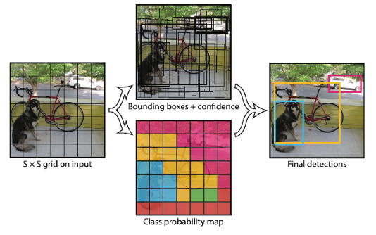
YOLO
- Split an images to S times S blocks.
- Apply object classification to each block and get confidence score of different objecxt for each block.
- Based on the class probability map to locate objects.
Calculation AP and mAP
- Gather Detection results
- Match Predictions to Ground Truth
- Compute Precision and Recall to generate a set of (recall, precision) points
- Build the Precision-Recall (PR) Curve (presioin decreases as recall increases)
- Smooth the Precision-Recall Curve
- Calculate AP
- Extend to mAP