Eunkwang Shin

Architecture​

Wall Detection​

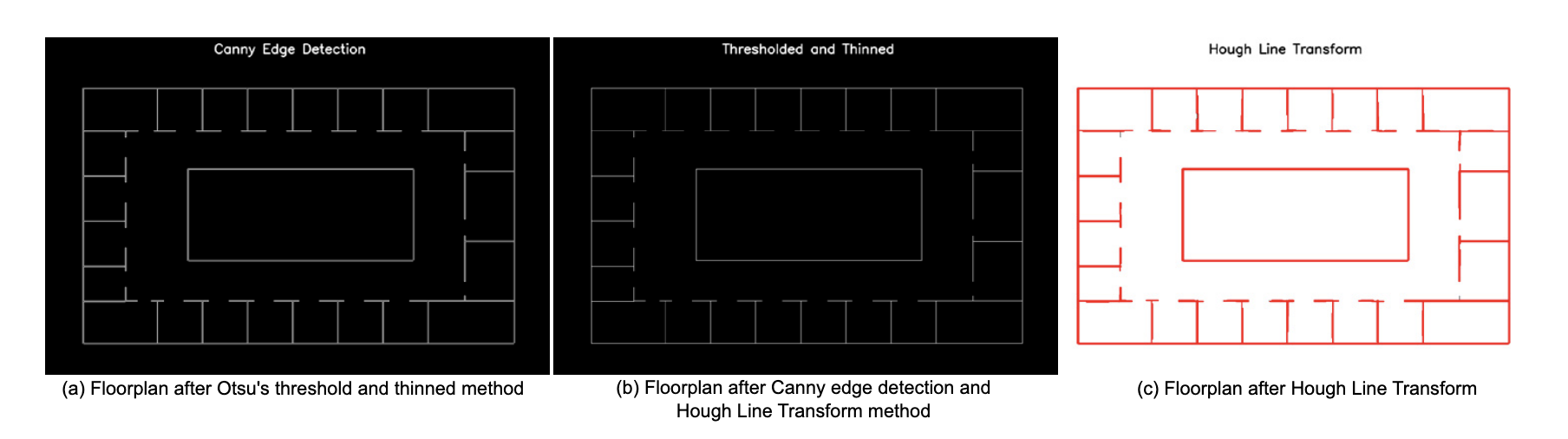
1. Pre-process floor images to gray scale.
2. Apply Otsu's threshold and thinned method.
3. Enhance the contrast of wall lines using Canny edge detection.
4. Employ Hough Transform to detect and map wall lines.

3D Visualization​

Limitations​

• Building structural details are unavailable or drone operations are restricted.
• Highly irregular floor plans or buildings constructed with unique materials not extensively represented in the training data.
• Real-time data integration
• Refined deep learning architectures, and validation across varied building materials and layouts
• Enhance the framework’s scalability and practical utility.

Spider GAN​

Sample

{
  "nodes": [
    { "id": 0, "name": "Drone",   "type": "source",   "features": [1, 0, 0, 0, 0.0] },
    { "id": 1, "name": "Room1",   "type": "room",     "features": [0, 1, 0, 0, -70.0] },
    { "id": 2, "name": "Room2",   "type": "room",     "features": [0, 1, 0, 0, -75.0] },
    { "id": 3, "name": "Room3",   "type": "room",     "features": [0, 1, 0, 0, -80.0] },
    { "id": 4, "name": "Corridor","type": "corridor", "features": [0, 0, 1, 0, -72.0] },
    { "id": 5, "name": "Wall_R1_R2","type": "wall",  "features": [0, 0, 0, 1, 0.0] },
    { "id": 6, "name": "Wall_R2_R3","type": "wall",  "features": [0, 0, 0, 1, 0.0] }
  ],

  "edges": [
    { "source": 0, "target": 1, "attenuation_db": 5.0  },
    { "source": 1, "target": 5, "attenuation_db": 8.0  },
    { "source": 5, "target": 2, "attenuation_db": 8.0  },
    { "source": 2, "target": 6, "attenuation_db": 10.0 },
    { "source": 6, "target": 3, "attenuation_db": 10.0 },
    { "source": 2, "target": 4, "attenuation_db": 3.0  }
  ]
}

Ref​

• Hason Rudd, D., Sanin, C., En, K. M., Gao, X., Islam, M. R., Hasan, M., Wang, X., Huo, A., & Xu, G. (2025). Location-Aware Deep Neural Network for Predicting Indoor 5G RSSI and CQI Using Drone-Based External RF Sensing. Procedia Computer Science, 270, 4765–4775. https://doi.org/10.1016/j.procs.2025.09.602

Vocabulary & Expressions​

Structural Knowledge​

• Structural knowledge: the relationship between concepts and objects in the world.
• Hierarchical approach: built on classification and uses hierarchies as the structures for knowledge representation, presented in a graphical format.
  • Semantic networks: nodes represent concepts, and edges represent relationships between concepts.
  • Ontologies
    • A formal specification of concepts, relationships, and constraints within a domain that enables machines to reason automatically.
    • It defines classes (concepts), subclasses (hierarchical relations), and properties (attributes or relations) that describe how entities interact.
    • Unlike simple taxonomies, ontologies also include logical axioms and constraints that specify allowable relationships and permit inference and consistency checking through automated reasoning.
    • Classes: Main concepts or categories (e.g. Person, Animal).
    • Subclasses: Subcategories (e.g. Dog ⊂ Animal).
    • Properties: Attributes (e.g. hasPart, hasColor).
    • Relations: Connection rules (e.g. MemberOf, SubsetOf).
    • Constraints: Logical constraints (e.g. disjointness, transitivity) that enable inference.

Requirement of hierarchices​

• Inclusiveness: Dog ⊆ Mammal ⊆ Animal
• Species/differentia: Dog = Mammal + (barks, canine traits, etc.)
• Inheritance: Mammal: has_fur, gives_live_birth → Dog: inherits all Mammal properties
• Transitivity: If Dog ⊆ Mammal and Mammal ⊆ Animal, then Dog ⊆ Animal
• Systematic and predictable rules for association and distinction
• Mutual exclusivity: Reptile ∩ Mammal = ∅
• Necessary and sfficient criteria:
  • Necessary: $\forall x,\ \text{Mammal}(x) \Rightarrow \text{Vertebrate}(x) \land \text{ProducesMilk}(x)$
  • Sufficient: $\forall x,\ \text{Vertebrate}(x) \land \text{ProducesMilk}(x) \Rightarrow \text{Mammal}(x)$

Advantage of hierarchical approach​

• Inferring from incomplete evidence (if the shared criteria are not obvious or easily observable).
  • Animal → Mammal → Dog: If an entity is classified as a Mammal, we can infer properties such as having fur and giving live birth, even if the entity is not explicitly identified as a Dog.
• Excellent representations in mature domains
  • Domains where entities and relationships are well understood and stable
  • e.g. medical diagnosis, biological taxonomy, type systems in programming languages.
• Useful for entities that are well defined and have clear class boudnaries.
  • Good fit: HTTP status codes, chemical elements, and biological species
  • Poor fit: emotions, social roles, and cultural practices
• Some theory or model is necessary to guide the identification
  • Provides criteria for defining entities and relationships
  • e.g. Evolutionary theory in biological taxonomy, Type theory in programming languages

Partition​

A partition of a category is a set of subcategories that form a disjoint, exhaustive composition of that category.

• Disjoint: Two or more categories are disjoint if they don't share common members.
• Exhaustive composition: The subcategories together cover all members of the parent category, leaving no member unclassified.
• Examples:
  • ❌ Category: Animal (Not a partition)
    • Mammal, Bird (Reptiles, fish, insects are missing, not exhaustive)
  • ✅ Category: Integer (Partition)
    • Even, Odd (Disjoint and exhaustive)

Physical composition​

• PartOf Relation: Partof(a, b) is a relation representing that one thing, 'a', is a part of another thing, 'b'.
• BunchOf Relation: BunchOf(a) is a relation, taking a set of objects 'a', to represent a composite object made up of those parts.
• Examples:
  • Partof(Wheel, Car): A wheel is part of a car (one-to-one relation).
  • BunchOf({Wheel1, Wheel2, Wheel3, Wheel4}): A car is a bunch of four wheels (many-to-one relation).
• Link between PartOf and BunchOf:
  • $\forall x (x \in s \implies PartOf(x, BunchOf(s)))$
  • $\forall y \Big[\big(\forall x (x \in s \implies PartOf(x, y)\big) \implies PartOf(BunchOf(s), y)\Big]$
• Why useful?
  • Reasoning from individual parts -> group -> larger object.
  • Avoiding ambiguity between: "this thing is part of", "these things together form"
  • Without BunchOf, ontologies cannot represent: piles, colleciton, aggregates, composite physical structures.

Measurements​

• Quantitive measures (Ratio, Interval)
  • Represented as numbers with units
  • Support arithmetic and unit conversion
  • Enable numeric reasoing (e.g. 2.54cm = 1 inch)
• Non-quantitative measures (Ordinal)
  • Cannot be meaningufully represented as numbers
  • Can still be compared using ordering relactions (<, >, =)
  • Suppor qualitative reasoning (e.g. one task is more difficult than another)

Objects​

• Stuff
  • Represents substances
  • Uncountable masses
  • Definitions include only intrinsic properties (e.g. Butter, Unsalted Butter)
  • $b \in Butter \land PartOf(p, b) \implies p \in Butter$
• Things
  • Represents discrete objects
  • Countable entities
  • Definitions include extrinsic properties (e.g. PoundOfButter, StickOfButter)
    • It depends on measurement
    • It depends on contextual constraints

Time​

• Fluent: a condition whose truth value can change over time.
  • e.g. "The box is on the table", $On(box, table)$, $On(box, table, t)$
  • a time-dependent proposition.
• Time scale and absolute time
  • Ontology represents time along a single continuous timeline with a fixed reference point.
  • $Date(0, 20, 21, 24, 1, 1995) = Seconds(300000000)$
  • It allows arithmetic operations on time and comparisons between time points.
• Time intertvals
  • Time can be represented as moments (instants) or intervals (durations).
  • $Duration(i) = Time(End(i)) - Time(Start(i))$
• Partition of time
  • $Partition({Moments, ExtendedIntervals}, Intervals)$
  • All time intervals can be partitioned into moments and extended (non-zero-length) intervals.
  • It provides a complete and precise ontology of time.

Event calculus​

• $T(f, t_1, t_2)$: Fluent $f$ is true for all time between time $t_1$ and $t_2$.
• $Happens(e, t_1, t_2)$: Event $e$ start at time $t_1$ and ends at time $t_2$.
• $Initiate(e, f, t)$: Event $e$ causes fluent $f$ to become true at time $t$.
• $Terminates(e, f, t)$: Event $e$ causes fluent $f$ to cease to be true at time $t$.
• $Initiated(f, t_1, t_2)$: Fluent $f$ becomes true at some point between $t_1$ and $t_2$.
• $Terminated(f, t_1, t_2)$: Fluent $f$ ceases to be true at some point between $t_1$ and $t_2$.
• $t_1 < t_2$: Time point $t_1$ occurs before time point $t_2$.
• Happens(PutBoxOnTable, 10, 12)
• Initiate(PutBoxOnTable, On(Box, Table), 12)
  • Initiated(On(box, table), 10, 12)
• T(On(Box, Table), 12, 20)
• Terminates(RemoveBoxFromTable, On(Box, Table), 20)
  • Terminated(On(box, table), 18, 22)

Successor-state axiom​

후속상태공리

• Define how the world changes after an action occurs.
  • what changes when an action happens
  • what stays the same.
• Without successor-state axioms, we face the frame problem:
  • after every action, we would need to explicitly list all facts that did not change.
• $Move(A, B, X)$: moving block A from the top of block B to position X.
  • Preconditions:
    • $On(A, B)$: A is on top of B
    • $Clear(A)$: nothing is on top of A
    • $Clear(X)$: nothing is on position X
  • Effects:
    • $On(A, X)$: A is now on position X
    • $Clear(B)$: B is now clear
    • $Clear(X)$: X is no longer clear (X is now occupied by A)

Semantic networks​

• Visually represent a knowledge base.
• Support efficient inference.
• Allow properties of an object ot be inferred from its category membership.
• Representing individual objects, categories of objects, and relations among objects.
• Categories are the primary buildling blokcs of large-scale knowledge representation schemes.

Taxonomy hierarchy​

• A hierarchical structure of categories
• Each lower category is a more specific kind of its parent
• Organized from general → specific

University Ontology​

Knowledge graph​

• represents information and its relationships using a graph structure.
• Nodes: entities or concepts (e.g. people, places, things).
• Edges: relationships between nodes (e.g. "is a", "part of", "located in").

Types of Knowledge Graphs​

• General Knowledge Graphs
• Domain-Specific Knowledge Graphs
• Semantic Knowledge Graphs
• Social Knowledge Graphs
• Temporal Knowledge Graphs
• Special Knowledge Graphs
• Statistical Knowledge Graphs
• Probabilistic Knowledge Graphs
• Textual Knowledge Graphs
• Multi-modal Knowledge Graphs

General Knowledge Graphs​

• Comprehensive information representation
• Entity-Relationship Structure
• Linked Data
• Semantic Enrichment
• Capabilities & Use Cases
  • Querying and Analysis
  • Data Integration
  • ML and AI applications

Examples​

• DBPedia: RDF, resource descritions framework
• Wikidata
• YAGO
• Google Knowledge Graph
• Microsoft Academic Graph
• IBM Watson Knowledge Studio

Reasoning for categories​

• Infer the presence of certain objects from perceptual input
• Infer category membership from perceived properties
• Use category information to make predictions
• It enables an agent to identify objects from observed properties and to predict further characteristics using category knowledge.

Reasoning using Semantic networks​

• Semantic networks are:
  • systems designed specifically for organizing categories reasoning with categories.
  • Provide graphical representations of a knowledge base
• Using a semanctic network, reasoning can be performed based on:
  • relationships between objects
  • category membership
  • inheritance between categories
  • properties associated with categories
  • Allows an object to inherit general knowledge from its category.
• The inheritance algorithm:
  • Starts from the object itself
  • Follows links upwards through the category hierarchy
  • Stops as soon as it finds a value for the property
  • This suppors efficient reasoning, default values, and exception handling.

RDF​

Resource Description Framework (RDF)

• Triple Structure: subject -> predicate -> object
• Subject: represents the resource being described or identified by a URI.
• Predicate (or Property): desribes the relationship between the subject and the object. also represented by a URI.
• Object: represents the value or target of the relationship. It can be a URI or a literal (a string, number, or date).

Uncertain Domain​

• Agent may need to handle uncertainty
• Environment is partially observable
  • Fully observable: An agent knows where it is.
  • The drone never knows its exact position, only an estimated one.
  • The true user intent is not directly observable, only noisy speech data.
  • It cannot see the whole environment or detect humans perfectly.
  • The true health state (disease present or not) is hidden.
• Environment is non-deterministic
  • AI Trading Agent
    • even if the agent takes the same action, the outcome can vary dramatically.
    • from market prices changes unpredictably due to external events (news, other traders, economic data).
    • network latency, competing traders' behavior are stochasic and independent, random fluctuations can affect the outcome.
    • buy action could lead to profit, loss, or no change depending on uncontrollable external factors.
  • AI Helpdesk Chatbot
    • even when the chatbot executes the same action, it sends queries to multiple backend systems, the result may differ each time.
    • network latency or failures, backend load, concurrent requests, and external dependencies can lead to different response times or outcomes.
    • same command doesn't guarantee the same outcome.
• Autonomous Driving
  • Partial Observability
    • Sensors cannot detect everything, blind spots, weather effects, occluded vehicles.
  • Non-Determinism
    • Even if the car signals a turn and starts moving, other drivers might brake suddenly, pedestrians might cross unexpectedly, or traffic lights might malfunction.
    • depending on random external events.
• Medical Diagnosis & Treatment Assistant
  • Partial Observability
    • The patient's internal health state is not directly visible.
    • tests can be inaccurate or incomplete: false positives/negatives, missing data
  • Non-Determinism
    • The same treatment can have different effects on different patients due to genetics, lifestyle, or random biological responses.
    • A drug may succeed, fail, or cause side effects.

Bayes' Theorem​

$P(A|B) = \frac{P(B|A) \cdot P(A)}{P(B)}$

• $P(A|B)$: Posterior probability, the probability of event A given taht B has occurred.
• $P(B|A)$: Likelihood, the probability of event B occurring given that A is true.
• $P(A)$: Prior probability, the initial probability of A being true before considering B.
• $P(B)$: Evidence, the total probability of B occurring.
• examples
  • 1% of people have a certain disease (prior probability). $P(Disease) = 0.01$
  • the test for the disease is 99% accurate (likelihood).
    • $P(PositiveTest|Disease) = 0.99$
    • $P(NegativeTest|NoDisease) = 0.99$
    • so $P(PositiveTest|NoDisease) = 0.01$
  • $P(PositiveTest) = P(PositiveTest|Disease) \cdot P(Disease) + P(PositiveTest|NoDisease) \cdot P(NoDisease)$
    • $= 0.99 \cdot 0.01 + 0.01 \cdot 0.99 = 0.0198$
  • $P(Disease|PositiveTest) = \frac{P(PositiveTest|Disease) \cdot P(Disease)}{P(PositiveTest)}$
    • $= \frac{0.99 \cdot 0.01}{0.0198} \approx 0.5$
• the conditional probability $P(effect|cause)$ quantifies the relationship in the causal direction from cause to effect.
• but $P(cause|effect)$ is often what we really want to know, describing the relationship in the diagnostic direction from effect to cause.
  • In medical dignosis, the doctor knows $P(symptoms|disease)$ from medical studies, and want to derive a $P(disease|symptoms)$ for a particular patient.
  • $P(disease|symptoms) = \frac{P(symptoms|disease) \cdot P(disease)}{P(symptoms)}$

General Form of Bayes' Rule​

$P(Y|X) = \alpha \cdot P(X|Y) \cdot P(Y)$

• $\alpha$ is the normalization constant needed to make the entries in $P(Y|X)$ sum to 1 for each value of X.
• conditional independency
  • two variables X and Y are conditionally independent given a third variable Z if the value of X provides no information about Y once Z is known.
  • $P(X, Y|Z) = P(X|Z) \cdot P(Y|Z)$

Constructing Bayesian Network​

• constructing a Bayesian network in which resulting joint probability distributions are a good representation of the agent's knowledge.
• 1. $P(x_1, ..., x_n) = \prod_{i=1}^{n} P(x_i | \text{parents}(x_i))$
• 2. rewrite the entries in the joint probability distribution in terms of conditional probabilities using the product rule.
  • $P(x_1 \land ... \land x_n) = P(x_n | x_{n-1} \land ... \land x_{1}) \cdot P(x_{n-1} \land ... \land x_{1})$
• 3. repeat step 2 until all variables are included.
  • $P(x_1, ..., x_n) = P(x_n | x_{n-1} \land ... \land x_{1}) \cdot P(x_{n-1} | x_{n-2} \land ... \land x_{1}) \cdots P(x_2 | x_1) \cdot P(x_1)$

Knowledge Representation​

• The agent's knowledge can at best provide only a degree of belief in the relevant logical sentences.
• A probabilistic agent may have a numerical degree of belief between 0 and 1.

Bayesian Network​

• a directed graph
• each node repressents a random variable and edge with an arrow from X to Y represents that X is a parent of Y.
• each node is associated with a probability distribution
• if a node Y has parents X, the Y node has a conditional probability distribution with respect to its parents X, i.e. $P(Y| \text{parents}(Y))$
• if a node has no any parents, it has an unconditional probability distribution.

Burglary Example​

• a new burglar alarm installed at home.
• it is reliable at detecting a burglary, but also responds on occasion to minor earthquakes
• you have two neighbors, John and Mary who promised to call you at work when they hear the alarm.
• given the evidence of who has or has not called, estimate the probability of a burglary.
• Knowledge representation as the probability of each event that can occur in this case.

$P(\text{event}_{j}) = \frac{\text{number of ccurrences of event }_j}{\text{total number of experiments}}$

• calulate the full joint probability distribution for all relevant variables.
  • specifying probabilities for all possible events one by one is unnatural and tedious.

$P(B, E, A, J, M) = \prod_{i}^{5} P(X_i | \text{parents}(X_i)) = P(B) \cdot P(E) \cdot P(A|B,E) \cdot P(J|A) \cdot P(M|A)$

$P(M, J, A, E, B) = P(B) \cdot P(E) \cdot P(A|B,E) \cdot P(J|A) \cdot P(M|A)$

Probabilistic reasnoing​

• to explain how to use network models to reason under uncertainty.
• Exact inference: calculate the exact posterior probabilities.
• Approximate inference: Stochastic approximation techniques such as likelihood weighting and Markov Chain Monte Carlo
  • can give reasonable estimates of the true posterior probabilities in a network
  • can cope with much larger networks than exact inference algorithms.
• Static worlds: Each random variable has a single fixed value.
• Dynamic worlds: view the world as a series of snapshots, or time slices.
  • Each of snapshots contains a set of random variables, some observed and some hidden.
  • The values of these variables can change over time.
  • With the assumption of state sequences are Markov, the future is independent of the past given the present.

Inference in Bayesian Networks​

• Computing the posterior probability distribution of a set of query variables, given some observed events, called some assignment of values to a set of evidence variables.
• $X$: query variable(s)
  • is it raining?
• $E$: the set of evidence variables with observed values $E_{1}, ..., E_{m}$
  • weather report says it is cloudy.
  • weather report says there is high humidity.
• $e$: a particular observed event.
  • $E_{1} = \text{cloudy}$
  • $E_{2} = \text{high humidity}$
• $Y$: the non-evidence, non-query variables.
  • the other variables in the network.
• $X = \{X\} \cup E \cup Y$
  • the complete set of variables in the network.
• $P(X|e)$: the posterior probability distribution of the query variable(s) given the evidence.
• $P(X|e) = \alpha \sum_{y} P(X, e, y)$

Exact inference in Bayesian Networks​

• One exact inference method is called by inference by enumeration.
• Observed some event $A = true$ and $B = true$, want to compute the posterior probability distribution $P(C|A, B)$.
  • Use the full conditional probability table
  • Use the Bayesian Network
• It calculates all the required probability components in each branch in the evaluation tree, and this results in repetitive calculations.
• To avoid this, we can use variable elimination algorithm and clustering algorithms.
• Calculation of probability distribution for a query variable is complexity exponential.
• Enumeration method can become intractable in large, multiple connected networks. -> use approximate inference methods.

For any Bayesian network with given nodes, $X = \{X_1, X_2, ..., X_n\}$, the joint probability distribution is given by: $P(X) = P(X_1 \land X_2 \land \ldots \land X_n) = \prod_{i=1}^{n} P(X_i | \text{parents}(X_i))$

Using the Bayesian network, we can compute the conditional probability.

$P(B | event) = \alpha \sum_{e}\sum_{a} P(B, E, A, j, m)$

• $i=1, P(X_1 | \text{parents}(X_1)) = P(B)$
• $i=2, P(X_2 | \text{parents}(X_2)) = P(E)$
• $i=3, P(X_3 | \text{parents}(X_3)) = P(A|B,E)$
• $i=4, P(X_4 | \text{parents}(X_4)) = P(j|A)$
• $i=5, P(X_5 | \text{parents}(X_5)) = P(m|A)$
• $P(B, E, A, j, m) = P(B) \cdot P(E) \cdot P(A|B,E) \cdot P(j|A) \cdot P(m|A)$

Berglary example calculation:

Bias​

• Bias quantifies how much on average the predicted values differ from the actual values.
• High bias implies the model is under-performing.

Variance​

• Variance quantifies how sensitive the model is to small changes in the training samples.

Ensemble Methods​

• The intuition behind ensemble methods is to decrease bias and variance by using multiple machine learning algorithms.
• Any machine learning algorithm can be used in ensemble methods.
  • decision trees, neural networks, logistic regressions, etc.
• Base models are as diverse as possible.
• Train each base model to predict as accurately as possible.

Sequential ensemble methods​

• Arrange weak learners in a sequence, such that weak learners learn from next learner in the sequence to create better predictive models.
• Each model fits the residual of its predecessor.

Parallel ensemble methods​

• to use different variations of the same dataset, of the smae classifier, and aggregate the results.

Bootstraping​

• Sampling technique that creates multiple subsets of datasets from the original dataset.
• when inferring results for a population from results found on a collection of smaller random samples of that population.

Bagging​

Bootstrap aggregating

• Generates subsets (bags) of traning data by sampling from the original training dataset with replacement.
• To overcome the complexity of models that overfit the training data.

Boosting​

• fits multiple models sequentially
• each model in the sequence is fitted giving more weight to the data points that were poorly handled by the previous models in the sequence.
• This process is iterated until the error function does not change, or the maximum limit of the number of estimators is reached.

Random Forest​

• Shallow trees have lower variance and higher bias, whereas deep trees have low bias but high variance.
  • Shallow trees are chosen for sequential ensemble methods
  • Deep trees are chosen for bagging methods (or parallel ensemble methods).
• a bagging method where deep trees are used and fitted on bootstrap samples, and then combined to produce an output with lower variance.
• selects randomly a set of features which are then used to decide the best split at each node of the tree.
• can be applied to both regression and classification tasks.
• can learn binary features, categorical features and numerical features.

1. create from the original dataset multiple bootstrap samples.
2. at each node in the decision tree, a random set of features is considered to decide the most beneficial split.
3. train a decision tree on each bootstrap sample.
4. final prediction is computed by averaging the prediction from all decision trees combined.

Advantages of Random Forest​

• generally accurate, quick to train
• can handle very large datasets
• can estimate importance of features
• generates an internal unbiased estimate of accuracy, which can use to know when to stop buildling
• can handle missing data
• can handle datasets with imbalanced classes
• can compute proximity between data points
• unsupervised for clustering and outlier detection

but don't handle large numbers of irrelevant attributes as well as some other methods.

Applications of Random Forest​

AdaBoost​

Adaptive Boosting

• simplest boosting algorithm, usaully uses decision trees for modelling
• multiple sequential models are created, each correcting the errors from the previous model.

GBM​

Gradient Boosting Machine

• works on both regression and classification problems.
• usually, regression trees are used as base models.

XGBoost​

eXtreme Gradient Boosting

• another implementation of gradient boosting algorithm.
• has proven to be a highly effective machine learning algorithm.
• extensively used in machine learning competitions due to its speed and performance.

Combining predictions​

Voting​

• Hard voting selection process uses predicted class labels for majority rule voting.
• Soft voting uses the predicted probabilities given by each base model, and the class label with the maximum sum of its probabilities is selected.
  • $\frac{1}{N} \sum_{i=1}^{N} P_{i}(c|x)$
  • where $N$ is the number of base models, and $P_{i}(c|x)$ is the probability predicted by model $i$ for class $c$ given input $x$.

Exception​

• Exeptions are throwable objects.
• Checked Exceptions are checked by the compiler and should be handled (thrown or caught).
• Unchecked or runtime Exceptions are not flagged by the compiler. Their occurrence during execution interrupts the program.
• Exceptions can be thrown by developers. Throwing an exception delegates handling the exception to a different class or different level of the program.
• Thrown exception is left not handled, it will cause runtime error.

Error​

• Java Errors usually indicate problems with the JVM or system resources.
  • it is not meant to be caught or handled by applications.
  • the base class is Error.
• Python is no separate Error class hierarchy. Errors are represented as exceptions.
  • ValueError, TypeError, MemoryError, SystemError, etc. are subclasses of Exception.

Java vs Pythone Exceiptions​

public class ExceptionExample {
    public static void main(String[] args) {
        Scanner scanner = new Scanner(System.in);
        try {
            System.out.print("Enter first number: ");
            int a = scanner.nextInt();
            System.out.print("Enter second number: ");
            int b = scanner.nextInt();
            int result = a / b; // This will raise ArithmeticException
            System.out.println("Result: " + result);
        } catch (ArithmeticException e) {
            System.out.println("Caught an exception: " + e.getMessage());
        } catch (NumberFormatException e) {
            System.out.println("Caught a number format exception: " + e.getMessage());
        } finally {
            System.out.println("This block always executes.");
        }
    }
}

def div(a, b):
    return a / b

a = input("Enter first number: ")
b = input("Enter second number: ")

try:
    result = div(int(a), int(b))  # This will raise ZeroDivisionError
    print("Result:", result)
except ZeroDivisionError as e:
    print("Caught an exception:", e)
except ValueError as e:
    print("Caught a value error:", e)
else:
    print("No exception occurred.")
finally:
    print("This block always executes.")

Throwing Exceptions​

class IncorrectAgeError(Exception):
    def __init__(self, age):
        self.age = age
        self.message = f"Age {age} is not valid. Age must be between 0 and 120."
        super().__init__(self.message)

number = int(input("Enter your age: "))

try:
    if number < 0 or number > 120:
        raise IncorrectAgeError(number)
    print(f"Your age is {number}.")
except IncorrectAgeError as e:
    print(e)

File Handlers​

• "r": Opens a file for reading, requires the file to exist
• "w": Opens a file for writing. If the file exists, it is truncated to zero length. If the file does not exist, a new text file is created.
• "a": Opens file for open for writing. The file is created if it does not exist.
• "+": Opens a file in updating mode (reading and writing). It can be used with reading (r+) and writing (w+) modes.
• "t": Opens a file in text mode (default mode).
• "b": Opens a file in binary mode. It can be used with reading (rb) and writing (wb) modes.

File Handler Methods​

os.path.exists("file.txt")  # Check if file exists
os.remove("file.txt")  # Delete a file
os.remove("dir")  # Delete an empty directory
os.chdir("path/dir")  # Change current working directory
os.getcwd()  # Get current working directory
os.mkdir("path/dir")  # Create a new directory

file_handler = open("file.txt", "r")  # Open a file in read mode
file_handler.read()  # Read the entire file content
file_handler.readline()  # Read a single line from the file
file_handler.close()  # Close the file

file_handler = open("file.txt", "w")  # Open a file in write mode
file_handler.write("Hello, World!")  # Write to the file
file_handler.write("\n")  # Write a newline character
file_handler.close()  # Close the file


import csv
with open("file.txt", "r") as file_handler:  # Using 'with' to handle file
    csv_object = csv.reader(file_handler)
    for row in csv_object:
        print(row)
    file_handler.close()

with open("file.txt", "a") as file_handler:  # Append mode
    csv_writer = csv.writer(file_handler)
    row = ["1", "gracefullight", "100"]
    csv_writer.writerow(row)
    file_handler.close()

import json
with open("data.json", "r") as file_handler:
    data = json.load(file_handler)  # Load JSON data from file
    print(data)
    file_handler.close()

with open("data.json", "w") as file_handler:
    json.dump(data, file_handler)  # Write JSON data to file
    file_handler.close()

• InputStream: reads byte-based input from various sources like files, memory, or network connections.
• OutputStream: writes byte-based output to various network connections.

Unit Testing​

• tests and verifies the smallest unis of an application such as functions, procedures, modules, or objects.
• the conducted during the development phase of the SDLC.
• Developers aim to identify defects and code bugs, which can save time and reduce costs in later testing stages.
• software testing encompasses the fourmain testing phases, and unit testing is at the foundational level of the process.
  • Unit Testing
  • Integration Testing
  • System Testing
  • Acceptance Testing

Python unit testing​

• test cases are defined using classes that inherit from unittest.TestCase
• assertions are used to validate results self.assertEquals()
• the unittest.TextTestRunner class can be used to run tests

import unittest

class TestMathOperations(unittest.TestCase):

    def test_addition(self):
        self.assertEqual(2 + 3, 5)

    def test_subtraction(self):
        self.assertEqual(5 - 2, 3)

    def test_multiplication(self):
        self.assertEqual(4 * 3, 12)

    def test_division(self):
        self.assertEqual(10 / 2, 5)

Knowledge representation​

• Intelligent agents need knowledge about the world in order to reach good decisions.
• Declarative knowledge is represented in a form of sentences in a knowledge representation language and stored in a knowledge base.
• Knowledge base is used by an inference engine to infer a new sentence which will be used for the agent to decide what action to take next.
• Formal languages are defined by its grammar and semantic rules
  • grammar: defines the syntax of legal sentences
  • semantic rules: defines the meaning.
• Common knowledge representation formalisms:
  • Propositional logic
  • First-order logic
  • Fuzzy logic
  • Semantic networks
  • Ontologies

Propositional logic​

• a declarative language in which can handle propositions that are known true, known false, or completely (unknown true or false)
• a BNK (Backus-Naur Form) grammer of sentences in propositional logic.
  • $\neg$ = NOT
  • $\land$ = AND
  • $\lor$ = OR
  • $\implies$ = IMPLIES
  • $\iff$ = IF AND ONLY IF
• Negation: a sentence using $\neg$ is called negation
• Literal: either an atomic sentence or a negated atomic sentence
• Conjunction: two sentences connected by $\land$. Eac hof them is called conjunct
• Disjunction: two sentences connected by $\lor$. Each of them is called disjunct
• Implication: two sentences connected by $\implies$. $P \implies Q$. P is called premise or antecedent and Q is the conclusion or consequent.
  • An implication is if-then statement.

Truth tables

FOL, First-order logic​

• a declarative language
• Syntax of FOL builds on that of propositional logic
• terms to represent objects, universal quantifier, and existential quantifier
• a model in FOL must provide the information required to determine the truth value of every atomic sentence in the language.
• $\forall x P(x)$ means for all x, P(x) is true
• $\exists x P(x)$ means there exists an x such that P(x) is true

Logical equivalence​

$\forall x \neg P(x) \equiv \neg \exists x P(x)$

• For all x, not P(x) is logically equivalent to "it is not the case that there exists an x such that P(x) is true."

Reasoning​

Deductive reasoning​

• a process of reasoning from one or more statements (premises) to reach a logical conclusion.
• first premise, second premise, therefore conclusion.

Inductive reasoning​

• the process of resoning from specific observations to borader generalizations and theories.
• also described as a method where one's experiences and observations are synthesized to cmoe up with a general truth.
• premises and then conclusion

Inference​

• steps in reasoning
• moves from premises to logical consequences
• In AI Context, inference is to derive new logical sentences (as the conclusion) from existing logical sentences (as premises).
• researchers develop automated inference systems to emulate human inference.

Inference Problem​

$KB \models \gamma$

• KB, Knowledge Base, is a set of propositions that represent what is known about the world.
• $\gamma$, Query sentence, is the target conclusion which needs to be confirmed based on the given KB.
• where $\models$ denotes the relation of logical entailment between KB and the sentence $\gamma$, reading as "KB entails $\gamma$" or "if KB is true, then $\gamma$ must also be true".
• $\alpha \models \beta \iff M(\alpha) \subseteq M(\beta)$
  • $M(\alpha)$ is the set of all models that satisfy $\alpha$.
  • $M(\beta)$ is the set of all models that satisfy $\beta$.
  • The statement $\alpha \models \beta$ means that in every model where $\alpha$ is true, $\beta$ is also true. In other words, if $\alpha$ holds, then $\beta$ must also hold.
• Model Checking: enumerates all possible models and checks if the entailment holds in each model.
  • Knowledge base will be used to draw inferences.
  • Query sentence, $\gamma$, is needed to be checked whether it is entailed by the KB.
  • Symbols, a list of all symbols (or atomic propositions) used in the problem context.
  • Models, assignments of truth and false values to those identified symbols.
• Model Checking Procedure
  1. Identify the propositional symbols involved in the KB sentences and query sentence
  2. Enumerate all possible models by assigning truth values to the identified symbols.
  3. Evaluate the KB sentence in each model and fined the models in which KB is true.
  4. Evaluate the query sentence in the models from step 3 and check if query sentence is true in these models.
  5. Conclude that the KB entails the query sentence $\gamma$ if and only if the query sentence is true in all models where the KB is true.

Inference Problem Example​

• Obersvation P: "It is raining"
• Query sentence Q: "The ground is wet"
• Knowledge: $P \implies Q$ (If it is raining, then the ground is wet)
• Knowledge Base KB: $P \land (P \implies Q)$
• Inference Problem: $KB \models Q$ from KB=T, get Q=T
• Proof:
  1. From the 4 possible models, only Model 1 makes KB true.
  2. M(KB) = model 1
  3. Model 1 also makes Q true.
  4. M(Q) = model 1
  5. $M(KB) \subseteq M(Q)$, therefore $KB \models Q$

Inference by theorem proving​

to apply rules of inference directly to the sentences in the KB to construct a proof of the desired sentence without consulting models.

• Proof: a chain of consequences that leads to the desired goal.
• KB will be used to draw inferences.
• Desired sentence is needed to be checked whether it is entailed by the KB.
• The rules of inference are the approved logical equivalences and rules.

Modus Ponens Rule​

$\frac{\alpha \implies \beta, \alpha}{\therefore \beta}$

• whenever any sentences of the form $\alpha \implies \beta$ and $\alpha$ are given, then the sentence $\beta$ can be inferred.

Add-Elimination Rule​

$\frac{\alpha \land \beta}{\therefore \alpha}$

• from a conjunction, one of the conjuncts can be inferred.

Terms to contradiction and resolution​

CNF
┌────────────────────────────────────────────────┐
│            (P ∨ Q)         ∧    (¬Q ∨ R)       │
│   ┌──────────────────────┐   ┌───────────────┐ │
│   │  Clause 1            │   │  Clause 2     │ │
│   │  (P ∨ Q)             │   │  (¬Q ∨ R)     │ │
│   │  ┌───────┬───────┐   │   │  ┌──────┬─────┐ │
│   │  │  P    │   Q   │   │   │  │ ¬Q   │  R  │ │
│   │  └───────┴───────┘   │   │  └──────┴─────┘ │
│   └──────────────────────┘   └───────────────┘ │
└────────────────────────────────────────────────┘

• Literal: an atomic sentence or its negation
• Complementary literals: a literal and its negation are complementary literals
• Clause: an expression formed from a collection of finite literals
  • In most $l_1 \lor l_2 \lor ... \lor l_n$ cases, a clause is a disjunction of finite literals.
  • written as the symbol $l_i$.
• Conjunctive Normal Form: a sentence expressed as a conjunction of clauses.
• Satisfiability: a sentence is satisfiable if it is true in, or satisfied by, some models.

Propositional satisfiability (SAT) problem​

• to determine the satisfiability of sentences in propositional logic.
• if there exists a model that satisfies a given logical sentence, then the sentence is satisfiable.
• Satisfiability can be checked by enumerating the possible models until one is found that satisfies the sentence, or by resolving complementary literals until an empty clause is derived.
• many problems in CS are really SAT problems.

Resolution rule​

Unit resolution rule​

$\frac{(l_1 \lor l_2 \lor ... \lor l_{i-1} \lor l_i \lor l_{i+1} \lor ... \lor l_k,\space m)}{l_1 \lor ... \lor l_{i-1} \lor l_{i+1} \lor ... \lor l_k}$

• where $l$ is a literal and $l_i$ and $m$ are complementary literals.
• Unit resolution rule takes a clause which is a disjunction of literals, and a literal and produces a new clause as the resolvent.

Full resolution rule​

$\frac{(l_1 \lor l_2 \lor ... \lor l_{i-1} \lor l_i \lor l_{i+1} \lor ... \lor l_k,\space m_1 \lor m_2 \lor ... \lor m_{j-1} \lor m_j \lor m_{j+1} \lor ... \lor m_n)}{(l_1 \lor ... \lor l_{i-1} \lor l_{i+1} \lor ... \lor l_k \lor m_1 \lor ... \lor m_{j-1} \lor m_{j+1} \lor ... \lor m_n)}$

• where $l$ is a literal and $l_i$ and $m_j$ are complementary literals.
• Full resolution rule takes two clauses which are disjuctions of literals and produces a new clause containing all the literals of the two original clauses except for the two complementary literals.

Inference via proof by contradiction through resolution​

$\alpha \models \beta$

• to prove that $\alpha \models \beta$, we can show that the sentence $\alpha \land \neg \beta$ is unsatisfiable.
• by deriving an empty clause $()$ from $\alpha \land \neg \beta$ using the resolution rule.
• In order to derive an empty clause, we use resolution which is a process to resolve complementary literals until to find an empty clause.
  1. R1: P (observation)
  2. R2: P $\implies$ Q (knowledge, raining implies ground is wet)
  3. $KB = P \land (P \implies Q)$
  4. Query sentence: Q
  5. Inference problem: $KB \models Q$, i.e. from $KB=T$, get $Q=T$
  6. Proof:
  • Let $(P \land (P \implies Q)) \land \neg Q$ valid
  • Convert $(P \land (P \implies Q)) \land \neg Q$ to CNF
  • Apply implication elimination rule, one has $(P \land (\neg P \lor Q)) \land \neg Q$
    • $C_1: P$
    • $C_2: \neg P \lor Q$
    • $C_3: \neg Q$
  • Apply unit resolution rule to $C_1$ and $C_2$, resolve $P$ and $\neg P$, one has $C_4: Q$
  • Apply unit resolution rule to $C_3$ and $C_4$, resolve $Q$ and $\neg Q$, one has $C_5: ()$

Inference in FOL​

• convert the first-order inference to propositional inference using the ruls for quantifiers.
  • universal instantiation (UI)
  • existential instantiation (EI)
• do inference in propositional logic using the methods about inference in propositional logic.
• this approach to first-order logic inference via propositionalization is complete, means any entailed sentences can be proved.
  • in most cases, this approach works
  • in some cases, it is slow and only useful when the domain is small.
• get rid of quantifiers by instantiating them with specific constants or variables.

Universal instantiation (UI)​

$\frac{\forall v \space \alpha}{\text{Subst}(\{v/g\},\alpha)}$

• to convert sentences with universal quantifiers to sentences without universal quantifiers.
• it can infer any sentence obtained by substituting a ground term for the universally quantified variable.
• $Subst(\{\theta, \alpha\})$ denotes the result of applying the subsitution $\theta$ to the sentence $\alpha$ and $g$ is a ground term or a constant symbol.
• universal instantiation can be applied many times to produce may different consequences.
• $\forall x Loves(x, Mary)$
  • $Loves(John, Mary)$
  • $Loves(Sue, Mary)$
  • $Loves(Bill, Mary)$
  • ...