RL 005

MDP

$(\mathcal{S}, \mathcal{A}, \mathcal{P}, \mathcal{R}, \gamma)$

• At each time step $t$, the agent observes state $S_t \in \mathcal{S}$ and chooses action $A_t \in \mathcal{A}$
• Receives reward $R_{t+1} \in \mathcal{R}$
• Transitions to a new state $S_{t+1}$

Transition Dynamics

Transition Probability

• How the environment responds to an action, independent of the agent's policy
• Policy: Whether to brake or accelerate when the traffic light is yellow.
• Transition Dynamics: How much the car decelerates after braking, and what the resulting next state is.

$P(s'|s,a) = P(S_{t+1} = s'|S_t = s, A_t = a)$

Policy

• A policy is the agent’s rule for choosing actions.
• It tells the agent what action to take in a given state.
• It defines agent's behavior.

$\text{Deterministic Policy}: \pi(s) = a$

• Direct mapping, and no randomness
• All probability on one action

$\text{Stochastic Policy}: \pi(a|s) = P(A_t = a | S_t = s)$

• A probability distribution over actions.
• More general, all four Bellman Equations are stochastic, use $\pi(a|s)$ to represent the policy.
• Policy is what the agent controls.

Value Functions

$v_\pi(s) = \mathbb{E}_\pi[R_{t+1} + \gamma v_\pi(S_{t+1}) | S_t = s]$

• How good is this state?
• $\mathbb{E}_\pi[G_t | S_t = s]$

$q_\pi(s,a) = \mathbb{E}_\pi[R_{t+1} + \gamma v_\pi(S_{t+1}) | S_t = s, A_t = a]$

• How good is this action in this state?
• $\mathbb{E}_\pi[G_t | S_t = s, A_t = a]$

$v_\pi(s) = \sum_{a \in \mathcal{A}} \pi(a|s) q_\pi(s,a)$

• The average value of the actions, weighted by the probability of choosing each action.
  • $a_1$ is brake
  • $a_2$ is accelerate
  • $v_\pi(s) = 0.8 * 10 + 0.2 * 20 = 10$

$$q_\pi(s,a) = \mathcal{R}(s,a) + \gamma \sum_{s' \in \mathcal{S}} P(s'|s,a) v_\pi(s')$$

• The value of taking action $a$ in state $s$: the immediate reward plus the discounted expected value of the possible next states.

Four Types of Bellman Equations

$$\begin{aligned} &v_\pi(s) = \sum_{a} \pi(a|s) q_\pi(s,a) \\ &q_\pi(s,a) = \mathcal{R}(s,a) + \gamma \sum_{s'} P(s'|s,a) v_\pi(s') \\ &v_\pi(s) = \sum_{a} \pi(a|s) \left[ \mathcal{R}(s,a) + \gamma \sum_{s'} P(s'|s,a) v_\pi(s') \right] \\ &q_\pi(s,a) = \mathcal{R}(s,a) + \gamma \sum_{s'} P(s'|s,a) \sum_{a'} \pi(a'|s') q_\pi(s',a') \end{aligned}$$

• Evaluate a state: $v_\pi(s)$
• Evaluate an action: $q_\pi(s,a)$
• Calculate Bellman by only $v$: Third equation
• Calculate Bellman by only $q$: Fourth equation

Dynamic Programming

Optimization method for sequential problem

• Dynamic: Sequential or Temporal component
• Programming: Optimizing a program or policy

• Sub Problem
• Optimal Solution

Prediction and Control

• Prediction: Evaluate a given policy $v_\pi(s)$
• Control: Find the optimal policy $\pi_*$

Policy Improvement

• $\pi \to v_\pi \to \pi'$
• $\pi' = \text{greedy}(v_\pi)$
• Evaluate current policy, Improve it greedily, then get a better policy

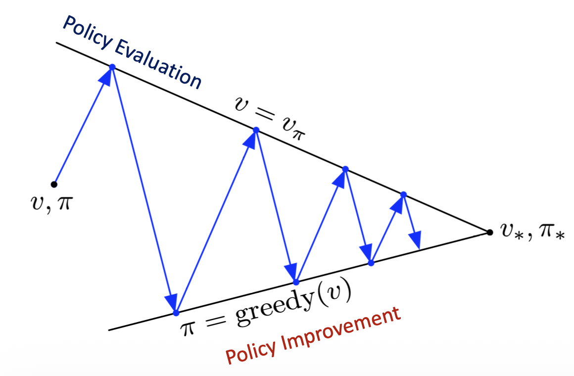
Modified Policy Iteration

• Policy iteration can be computationally expensive
• MPI: cut off the policy evaluation after a few iterations $k$ then step to policy improvement.
  • $k = 1 \Rightarrow \text{Value iteration}$
  • $k = 3,4 \Rightarrow \text{Modified Policy iteration}$
  • $k \quad \text{is large enough} \Rightarrow \text{Policy iteration}$

Poisson Distribution Formulation

$P(X = n) = \frac{\lambda^n e^{-\lambda}}{n!}$

• How many times an event occurs within a fixed interval of time (or space) when we only know the long-term average rate ($\lambda$).
• $n$: The actual number of requests or returns ($n \in \{0, 1, 2, \ldots\}$)
• $\lambda$: The expected/average number of requests or returns
• $e$: Euler's number (2.71828)
• $n!$: Factorial of $n$

Deterministic Value Iteration

$v_*(s) = \max_{a} \left( \mathcal{R}(s,a) + \gamma \sum_{s'} P(s'|s,a) v_*(s') \right)$

• If solutions to sub-problems $v_*(s')$ are known, the optimal value $v_*(s)$ for the current state can be computed directly.
• Value signals propagate backwards across the state space from states with terminal rewards.

Value Iteration

$v_{k+1}(s) = \max_{a} \left( \mathcal{R}(s,a) + \gamma \sum_{s'} P(s'|s,a) v_k(s') \right)$

• Infinite ($\infty$) iterations are required to converge exactly to $v_*$.
• In practical implementations, iteration terminates when the maximum value change between iterations is less than a small threshold $\theta$.

Dynamic Programming ALgorithms

Problem	Bellman Equation	Algorithm
Prediction	Bellman Expectation: $v_{k+1}(s) = \sum_{a \in A} \pi(a \mid s) \left( R(s, a) + \gamma \sum_{s' \in S} P(s' \mid s, a) v_k(s') \right)$	Iterative Policy Evaluation
Control	Bellman Expectation + Greedy Policy Improvement: $v_{k+1}(s) = \sum_{a \in A} \pi(a \mid s) \left( R(s, a) + \gamma \sum_{s' \in S} P(s' \mid s, a) v_k(s') \right)$ $\pi' = \text{greedy}(V_\pi)$	Policy Iteration
Control	Bellman Optimality: $v_{k+1}(s) = \max_a \left( R(s, a) + \gamma \sum_{s' \in S} P(s' \mid s, a) v_k(s') \right)$	Value Iteration

Efficiency of DP

• Strengths:
  • A foundational and efficient framework widely used for solving MDPs.
  • Mathematically guaranteed to converge to an optimal policy in polynomial time in terms of the number of states and actions.
  • Exponentially faster than exhaustive direct search across the policy space ($|A|^{|S|}$).
• Limitations:
  • Can become computationally impractical for extremely large or complex environments.
  • Curse of Dimensionality: As the number of state variables (dimensions) increases, the total state space size ($|S|$) expands exponentially, leading to severe computational and memory bottlenecks.

Asynchronous Dynamic Programming

• Comparison with Synchronous Methods: Standard DP methods sweep through the entire state space systematically in every iteration. Asynchronous DP backs up individual states independently in arbitrary order.
• In-place Value Updates: Directly overwrites values in a single memory array, allowing immediate propagation of newly updated state values to subsequent calculations.
• Computational Gain & Convergence:
  • Significantly reduces computation by avoiding exhaustive full-state sweeps.
  • Guaranteed to converge to the optimal value function $v_*$, provided that all states continue to be selected and updated indefinitely.

Real-Time Dynamic Programming (RTDP)

• Interaction-Driven Online Updates: Solves sub-problems on-the-fly by focusing updates specifically on states that are directly relevant to the agent's current trajectory.
• Target Applications: Large-scale environments where full state-space iteration is intractable (e.g., robotics, autonomous control systems, game AI).
• Core Characteristics:
  • Online Decision Making: Makes and refines decisions while operating directly in the environment.
  • Lazy Evaluation: Computes values only for visited or critical state subsets rather than unvisited distant states.
  • Adaptive Exploration: Guides search toward high-reward trajectories through active interaction.
  • Approximate MDP Solution: Yields near-optimal policies for relevant regions without solving the global MDP.

Approximate Dynamic Programming (ADP)

• Motivation: Addresses the curse of dimensionality where tabular representation of states and exact value computation become computationally infeasible.
• Function Approximation Methods: Parameterizes and estimates the value function using scalable statistical and machine learning models:
  • Linear models, deep neural networks, decision trees, and general regression techniques.
• Error Management Mechanisms:
  • Eligibility Traces: Accelerates credit assignment and temporal consistency across multi-step transitions.
  • Experience Replay: Stores transition tuples in a replay buffer and samples them randomly to break data correlation and stabilize value approximation.