RL 004

Bellman Equation

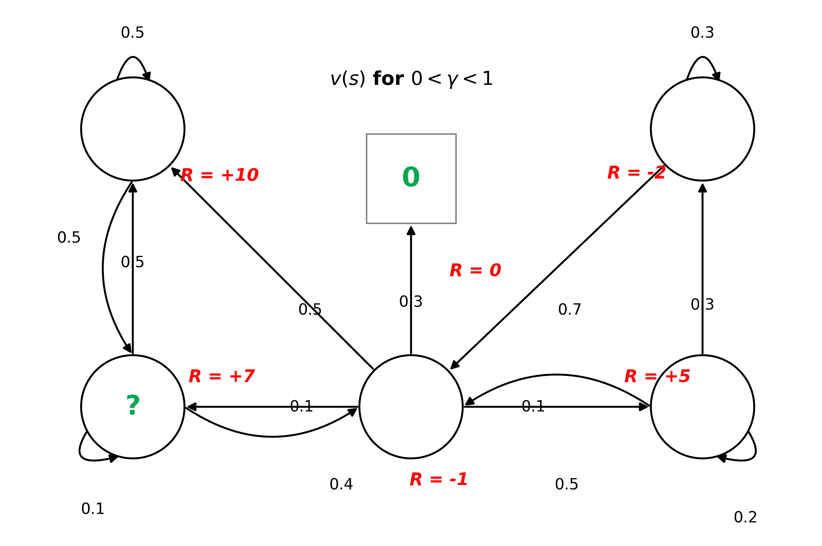
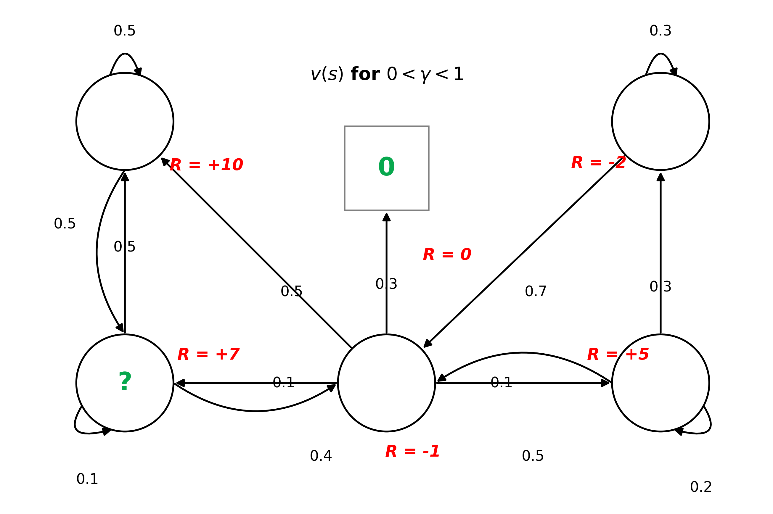
$v_\pi(s) = \mathbb{E}_\pi \left[ \underbrace{R_{t+1}}_{\text{Immediate Reward}} + \gamma \underbrace{v_\pi(S_{t+1})}_{\text{Discounted Future Value}} \;\middle|\; \underbrace{S_t = s}_{\text{Starting at state s}} \right]$

• Fundamental concept in RL using a recursive equation to express a way to compute the value of a state based on the values of its successor states.

$$\begin{aligned} v(s) &= \mathbb{E} \left[ R_{t+1} + \gamma R_{t+2} + \gamma^2 R_{t+3} + \dots \;\middle|\; S_t = s \right] \\[8pt] &= \mathbb{E} \left[ R_{t+1} + \gamma \underbrace{\left( R_{t+2} + \gamma R_{t+3} + \dots \right)}_{G_{t+1}} \;\middle|\; S_t = s \right] \\[8pt] &= \mathbb{E} \left[ R_{t+1} + \gamma G_{t+1} \;\middle|\; S_t = s \right] \\[8pt] &= \mathbb{E} \left[ R_{t+1} + \gamma v(S_{t+1}) \;\middle|\; S_t = s \right] \\[8pt] &= \underbrace{\mathbb{E}[R_{t+1} \mid S_t = s]}_{\text{Immediate Reward } \mathcal{R}(s)} + \gamma \, \underbrace{\mathbb{E}[v(S_{t+1}) \mid S_t = s]}_{\text{Expected Next State Value}} && (\because \mathbb{E}[X + \gamma Y] = \mathbb{E}[X] + \gamma\mathbb{E}[Y]) \\[10pt] &= \mathcal{R}(s) + \gamma \underbrace{\sum_{s'} \mathcal{P}(s' \mid s) v(s')}_{\text{Transition Dynamics}} && \left(\because \mathbb{E}[g(X)] = \sum_x P(x)g(x)\right) \end{aligned}$$

Bellman Equation Example

$v(s_{\text{BL}}) = 7 + \gamma(0.1 \cdot v(s_{\text{BL}}) + 0.5 \cdot(s_{TL}) + 0.4 \cdot(s_{BR}))$

Bellman Equation in Matrix Form

$v = \mathcal{R} + \gamma \mathcal{P} v$

$$\begin{aligned} \underbrace{ \begin{bmatrix} v(s_1) \\ \vdots \\ v(s_n) \end{bmatrix}}_{\text{V of a particular state}} = \underbrace{\begin{bmatrix} \mathcal{R}(s_1) \\ \vdots \\ \mathcal{R}(s_n) \end{bmatrix}}_{\text{Immediate Reward}} + \gamma \underbrace{\begin{bmatrix} \mathcal{P}_{11} & \cdots & \mathcal{P}_{1n} \\ \vdots & \ddots & \vdots \\ \mathcal{P}_{n1} & \cdots & \mathcal{P}_{nn} \end{bmatrix}}_{\text{Transition Matrix}} \underbrace{\begin{bmatrix} v(s_1) \\ \vdots \\ v(s_n) \end{bmatrix}}_{\text{V of future state}} \end{aligned}$$

Solving the Bellman Equation

Linear System of Equations

$$\begin{aligned} \mathcal{v} &= \mathcal{R} + \gamma \mathcal{P}\mathcal{v} \\ \mathcal{v} - \gamma \mathcal{P}\mathcal{v} &= \mathcal{R} \\ (I - \gamma \mathcal{P})\mathcal{v} &= \mathcal{R} \\ \mathcal{v} &= (I - \gamma \mathcal{P})^{-1} \mathcal{R} \end{aligned}$$

• Computational Complexity: $O(n^3)$
• For small MDPs: direct solution is possible (up to 100 states)
• For large MDPs:
  • Iterative methods
  • Dynamic Programming
  • Monte Carlo Tree
  • TD learning