RL 003

Markov Property

• The future is independent of the past given the present state.
• The current state is sufficient to determine the future, without history.

Markov State

$P[S_{t+1} | S_t] = P[S_{t+1} = s' | S_t = s]$

• $t$: Time step
• $S_{t+1}$: Next state
• $S_t$: Current state
• $S_1, \ldots, S_t$: History (All previous states)

State Transition Probability

$P_{ss'} = P[S_{t+1} = s' | S_t = s]$

• Likelihood or probability of moving from one state $s$ to another state $s'$ in the next time step $t+1$.
• $s$: Markov State
• $s'$: Successor State
• $t$: Time step
• State transition matrix $P$ defines the transitions probabilities between all states $s$ to all successor states $s'$.

State Transition Matrix

$$\mathcal{P} = \begin{array}{rl} & \begin{matrix} \textcolor{red}{\boldsymbol{s_1}} & \textcolor{red}{\boldsymbol{\dots}} & \textcolor{red}{\boldsymbol{s_n}} \end{matrix} \quad \leftarrow \text{(to state)} \\ \begin{matrix} \textcolor{red}{\boldsymbol{s_1}} \\ \textcolor{red}{\boldsymbol{\vdots}} \\ \textcolor{red}{\boldsymbol{s_n}} \end{matrix} & \hspace{-10pt} \begin{bmatrix} \mathcal{P}_{11} & \dots & \mathcal{P}_{1n} \\ \vdots & \ddots & \vdots \\ \mathcal{P}_{n1} & \dots & \mathcal{P}_{nn} \end{bmatrix} \\ \begin{matrix} \uparrow \\[-2pt] \mathclap{\text{(from state)}} \end{matrix} & \end{array}$$

• State transition matrix $P$ defines the transition probabilities between all states $s$ to all successor states $s'$.
• Probability of moving from state $s_n$ to $s_1$ is $\mathcal{P}_{n1}$.

Math cal

Reinforcement Learning and Math Major Symbols

• $\mathcal{P}$: Transition Probability Matrix
• $\mathcal{S}$: State Space
• $\mathcal{A}$: Action Space
• $\mathcal{R}$: Reward Function
• $\mathcal{L}$: Loss Function
• $\mathcal{N}(\mu, \sigma^2)$: Normal Distribution
• $\mathcal{D}$: Dataset
• $\mathcal{H}$: Entropy / Hypothesis Space

Markov Process

Markov Chain

• What is going to be happened next?
• it goes through a sequence of states overtime.
• Stochastic Process: The next state $S_{t+1}$ is determined by the current state $S_t$ and the transition probability matrix $P$ that exhibits the Markov Property.
• Current state is independent of the past states.
• Memoryless: History of states leading up to the current state is not necessary to predict the next/future state.
• MP: $\langle\mathcal{S},\mathcal{P}\rangle$, What states comes next?, Observer's Perspective.
• MRP: $\langle\mathcal{S},\mathcal{P},\mathcal{R},\gamma\rangle$, How good/How much reward is this state in the long run?, Evaluator's Perspective.
• MDP: $\langle\mathcal{S},\mathcal{A},\mathcal{P},\mathcal{R},\gamma\rangle$, What action should I take right now to maximize the long-term reward?, Decision Maker's Perspective.

$\mathcal{P}_{ss'} = P[S_{t+1} = s' | S_t = s]$

• $S$: a finite set of states.
• $\mathcal{P}$: a state transition matrix, defines the transitions probabilities from all states $s$ to all successor states $s'$.
• NO REWARD, NO ACTIONS.

Transition Diagram

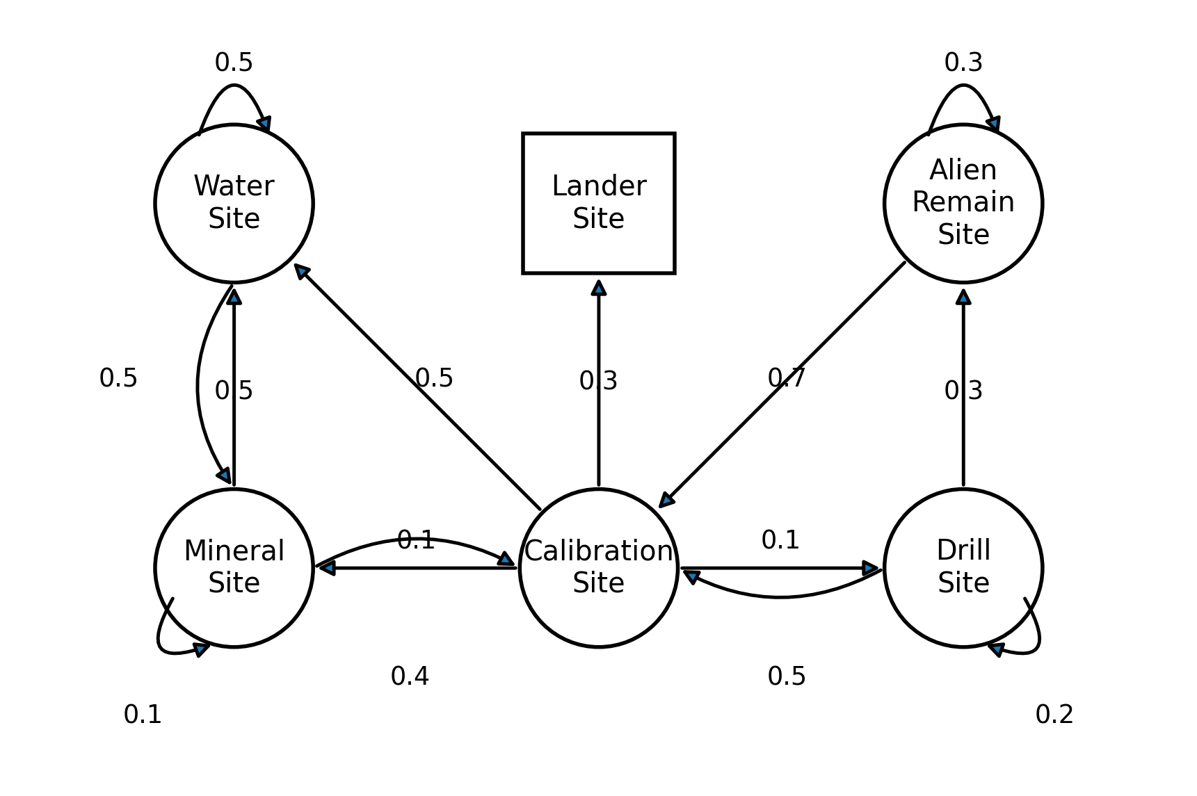
• Box: where it ends
• Arrow: transitions
• Circle: states
• Number: probability of transitioning to the state

$$\mathcal{P} = \begin{bmatrix} 0 & 0.1 & 0.5 & 0.1 & 0 & 0.3 \\ 0.4 & 0.1 & 0.5 & 0 & 0 & 0 \\ 0 & 0.5 & 0.5 & 0 & 0 & 0 \\ 0.5 & 0 & 0 & 0.2 & 0.3 & 0 \\ 0.7 & 0 & 0 & 0 & 0.3 & 0 \\ 0 & 0 & 0 & 0 & 0 & 1 \end{bmatrix}$$

• S1: Calibration Site
• S2: Mineral Site
• S3: Water Site
• S4: Drill Site
• S5: Alien Remain Site
• S6: Lander Site

Markov Chain Episode

• A sequence of states from a starting state to a terminal state.
• $S_1, S_3, S_2, S_1, S_6$
• $S_1, S_3, S_3, S_2, S_1, S_4, S_4, S_1, S_6$

Episodic Task vs Continuous Task

Feature	Episodic Tasks	Continuing Tasks
Termination	Has a well-defined terminal state ($T$)	Runs indefinitely without termination ($T = \infty$)
Real-World Examples	• Video games (e.g., Super Mario: level clear or death) • Navigation (reaching destination) • Board games (e.g., Chess: checkmate/draw)	• Smart thermostat (HVAC temperature control) • 24/7 industrial robotic process control • Automated trading & server load management
Execution Flow	Environment resets to a start state once finished	Operates continuously without automatic resets

• Episodic Tasks: Tasks with a defined end/terminal state.
• Continuing Tasks: Tasks without a defined end/terminal state.
• It may require different MDP formulation and solution methods for each type of task.

Markov Reward Process

Markov Chain + Reward

$\langle\mathcal{S},\mathcal{P},\mathcal{R},\gamma\rangle$

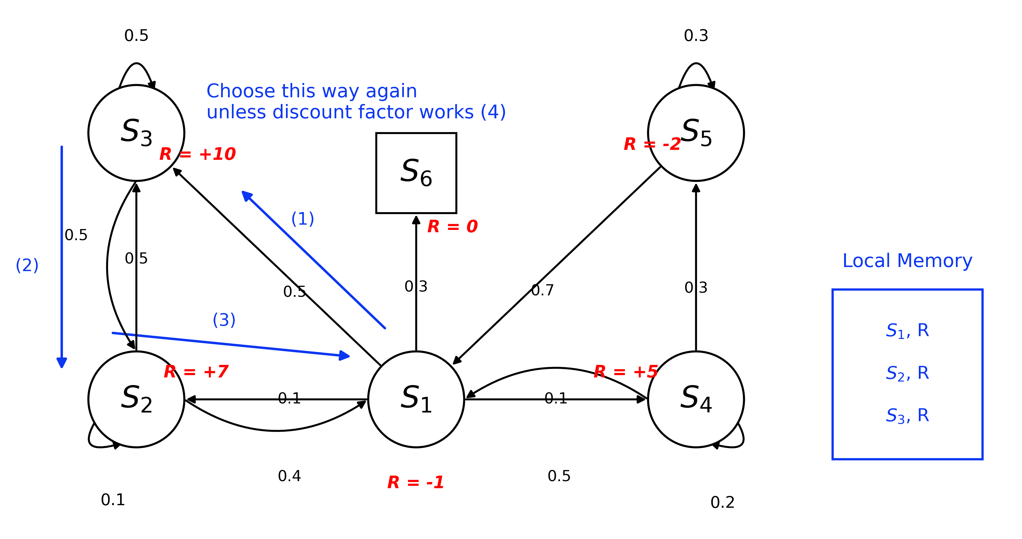
• $S$: a finite set of states.
• $\mathcal{P}$: a state transition matrix (Transition Dynamics)
• $\mathcal{R}$: a reward function to compute expected reward from a state.
  • $\mathcal{R}_s = \mathbb{E}[R_{t+1} | S_t = s]$
  • In the state $s$, how much reward can you expect to get in the next time step?
• $\gamma$: a discount factor, to balance the immediate and future rewards.
  • $\gamma \in [0, 1]$

Return

$G_t = R_{t+1} + R_{t+2} + \cdots + R_T$

• $G_t$: Goal Reward
  • The sum of the rewards received from time step $t$.
• $R_{t+1}, R_{t+2}, \ldots, R_T$: the sequence of rewards received after time step $t$
• $T$: terminal state
• $t$: time step

Discount

• The present value of future rewards.
• $\gamma = 0$: Myopic evaluation for maximizing immediate reward.
• $\gamma = 1$: Far-sighted/Long-term evaluation for maximizing future reward.

Discounted Return

$G_t = R_{t+1} + \gamma R_{t+2} + \gamma^2 R_{t+3} + \cdots + \gamma^{T-t-1} R_T = \sum_{k=0}^{\infty} \gamma^k R_{t+k+1}$

• $G_t$: Discounted Return
• $\gamma = 1$: Undiscounted Markov Reward Process, if all sequences terminate (like games)

Value Function

$v(s) = \mathbb{E}[G_t | S_t = s]$

• The expected return from state $s$.
• How much total reward can you expect to get starting from this state?
• A function returning the expected cumulative reward starting from state $s$

Markov Decision Process

Markov Reward Process + Actions(Decisions)

$\langle\mathcal{S},\mathcal{A},\mathcal{P},\mathcal{R},\gamma\rangle$

• $S$: a finite set of states.
• $\mathcal{A}$: a finite set of actions.
• $\mathcal{P}$: a state transition matrix
  • $\mathcal{P}_{ss'}^a = P[S_{t+1} = s' | S_t = s, A_t = a]$
• $\mathcal{R}$: a reward function
  • $\mathcal{R}_s^a = \mathbb{E}[R_{t+1} | S_t = s, A_t = a]$
• $\gamma$: a discount factor

Policy

$\pi(a | s) = P[A_t = a | S_t = s]$

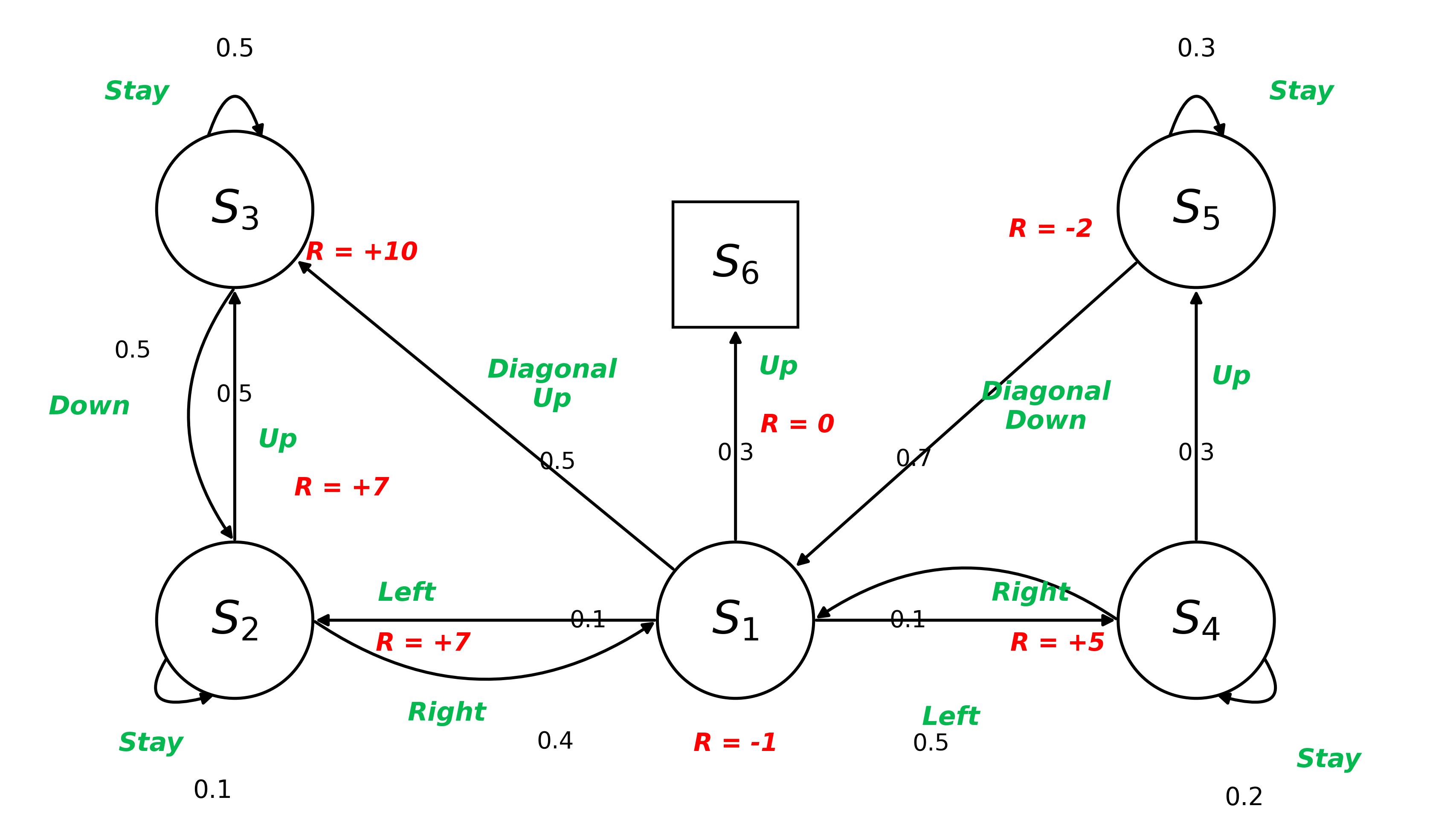
• Policy specifies what actions to take in each state.
  • $\pi(\text{left} | \text{wall}) = 0.8$
  • $\pi(\text{right} | \text{wall}) = 0.2$
  • $\pi(\text{straight} | \text{wall}) = 0.0$
  • The agent's playbook for any given state.
• It fully defines the behavior of the agent.
• MDP's policy does not depends on history, only on the current state.

Value Function of a Policy

$v_\pi(s) = \mathbb{E}_{\pi}[G_t | S_t = s]$

• The state value function $v_\pi(s)$ is the expected return starting from state $s$ and following policy $\pi$.
• How good it is to be in state $s$ (under policy $\pi$)?

$q_\pi(s, a) = \mathbb{E}_{\pi}[G_t | S_t = s, A_t = a]$

• The expected return of taking action $a$ in state $s$, taking action $a$ and then following policy $\pi$.
• $q$: a quality of action $a$ in state $s$ (under policy $\pi$).

Feature	State-Value Function ($v_\pi(s)$)	Action-Value Function ($q_\pi(s, a)$)
Decision Flow	Follows policy $\pi$ right from state $s$	Commits to action $a$ first, then follows policy $\pi$
Intuitive Question	"How good is it to be in this state?"	"How good is it to take this specific action in this state?"

Solving MDPs

Goal: Find optimal policy $\pi_*$ that maximizes the expected return.

• Using Value Iteration or Policy Iteration.
• Updating value functions and policies iteratively until convergence.
• Evaluation: Compute the value function $v_\pi(s)$ for a given policy $\pi$.
• Improvement: Update the policy $\pi$ to choose better actions based on the updated value function.
  • To converge to the optimal value function and policy $v^*, \pi^*$

POMDPs

MDPs with hidden states.

$\langle \underbrace{\mathcal{S}, \mathcal{A}, \mathcal{O}}_{\text{공간 (Spaces)}}, \underbrace{\mathcal{P}, \mathcal{R}, \mathcal{Z}}_{\text{함수 / 규칙 (Functions)}}, \underbrace{\gamma}_{\text{상수 (Discount Factor)}} \rangle$

• $S$: a finite set of states
• $\mathcal{A}$: a finite set of actions
• $\mathcal{O}$: a finite set of observations
  • e.g. driving in foggy weather.
• $\mathcal{P}$: a state transition matrix
• $\mathcal{R}$: a reward function
• $\mathcal{Z}$: an observation function
  • $\mathcal{Z}_{s', o}^a = P[O_{t+1} = o | S_{t+1} = s', A_t = a]$
  • an observation function specifying the probability of receiving observation $o$ given state $s'$ and action $a$
  • After taking action $a$ and landing in state $s'$, how likely is the agent to observe $o$?
• $\gamma$: a discount factor
• e.g.
  • Robot navigation with noisy/uncalibrated sensors.
  • Autonomous Driving with Sensor uncertainty due to bad weather conditions and unexpected events.

Finite Horizon MDPs

• Finite Time Steps ($T$): A sequential decision-making process restricted to a fixed, finite number of steps ($T$) to maximize cumulative rewards.
• Target Applications: Well-suited for problems with explicit deadlines or time-varying environment dynamics.
• Decision Basis: Optimal decisions are made using current state ($S_t$), available actions ($A_t$), transition probabilities ($\mathcal{P}$), and immediate rewards ($\mathcal{R}$).
• Representative Example: A robot navigating a grid world with a limited step count or battery budget to reach a goal while avoiding obstacles.
• Discount Factor ($\gamma$): Because the horizon $T$ is finite, the cumulative return cannot diverge to infinity, allowing the use of undiscounted formulations ($\gamma = 1$).
• Time-Dependent (Non-Stationary) Policy:
  • Unlike infinite-horizon MDPs, the optimal action depends explicitly on the remaining time steps ($T - t$).
  • Policy Notation: $\pi_t(s)$ (indexed by time step $t$).
  • Intuition: An agent may play conservatively early on, but take high-risk, high-reward actions right before the deadline.

Dimension	Finite-Horizon MDP	Infinite-Horizon MDP
Time Horizon ($T$)	$T < \infty$ (Explicit terminal step)	$T \to \infty$ (Perpetual / ongoing)
Policy Nature	Non-Stationary ($\pi_t(s)$, changes over time)	Stationary ($\pi(s)$, time-invariant)
Discount Factor ($\gamma$)	$\gamma \le 1$ ($\gamma = 1$ is valid)	Typically $\gamma < 1$ required for convergence
Objective Function	$\max \mathbb{E} \left[ \sum_{t=0}^{T} \gamma^t R_{t+1} \right]$	$\max \mathbb{E} \left[ \sum_{t=0}^{\infty} \gamma^t R_{t+1} \right]$

Limitations of MDPs

• Markovian Assumption: Assumes future transitions depend solely on the current state $S_t$, ignoring past historical trajectories and temporal dependencies that matter in real-world dynamics (e.g., momentum, acceleration).
  • State augmentation, frame stacking, RNN/Transformer, POMDP
• Complete Knowledge Requirement: Assumes exact a priori knowledge of transition probabilities $\mathcal{P}$ and reward functions $\mathcal{R}$, which are rarely accessible without sample-based learning in complex environments.
  • Model-free RL: Q-learning, SARSA, Policy Gradient
• Finite State and Action Spaces: Restricted to discrete and countable sets, whereas real-world robotics and physical control tasks typically involve continuous states and actions.
  • Function approximation, Actor-Critic: DDPG, TD3, SAC, PPO
• Curse of Dimensionality: Tabular value and policy storage scale exponentially as state dimensions grow ($|\mathcal{S}| \times |\mathcal{A}|$), making high-dimensional environments (e.g., raw pixel inputs) computationally intractable.
  • Deep RL: neural approximation of $V$, $Q$, or $\pi$
• Partial Observability: Assumes full access to the true ground-truth state ($O_t = S_t$), failing to account for real-world sensor noise, occlusions, and incomplete observations.
  • POMDP, belief-state estimation, recurrent policies