CNN 006

Data Preparation

• Small Dataset (Range: 100 to 100,000 samples)
  • Train/Valid/Test: 60/20/20
  • Train/Test: 70/30
• Large Dataset (Range: 500,000 to 1M+ samples)
  • Train/Valid/Test: 98%/10,000/10,000
  • usaully more traning data is get better performance.
• Rule of Thumb: Validation and Test set should com from the same distribution.

Bias and Variance

• Bias: A value that allows to shift the activation function to left or right to better fit the data.
  • With bias the curve/line will not always pass through origin
  • can get a better fit to training data
• Variance: The sensitivity of the model to small fluctuations in the training data.
  • The change in prediction accuracy of ML model between training data and test data.
  • Model with high variance pays a lot of attention to tranining data and does not generalize on the data which is has not seen before.
  • With high variance, model perform very well on training data but poorly on test data.

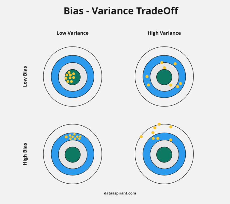
• High Bias
  • High training error, underfitting
  • Validation/test error nearly same as train error
  • Potential things to try:
    • Increase features
    • Make ML model more complicated
    • Decrease Regularation parameters
• High Variance
  • Low tranining error, overfitting
  • High validation/test error
  • Potential things to try:
    • Increase dataset size
    • Reduce input features
    • Increasing Regularization parameter

Accuracy

• Bayesian Optimal Error (BOE): Best optimal error that can be achieved by any model on a given dataset.
• Human-Level performance:
  • Humans are very good at a lot of tasks
  • Can get labelled data from humans to help improve the model performance
  • Gain insights from manual error analysis

Regularization

• a technique which makes slight modifications to the learning algorithm such that the model generalizes better on the unseen data.
• Update the loss/cost function by adding a regularization term
  • $\text{Loss function} = \text{Loss} + \text{Regularization term}(\lambda)$
  • Due to $\lambda$, the weight matrices will decrease, assuming a neural network with smaller weight matrices leads to simpler model.
  • Regularization penalizes the weights matrices of the nodes
• L2 regularization
• L1 regularization
• Dropout

L2 Regularization

$\text{Cost function} = \text{Loss} + \frac{\lambda}{2m} \sum_{j=1}^{n_x} w_j^2$

• $\lambda$ is a hyper-parameter
• as weight decay, as it forces the weight to decay towards zero, but not exactly zero.

L1 Regularization

$\text{Cost function} = \text{Loss} + \frac{\lambda}{2m} \sum_{j=1}^{n_x} |w_j|$

• Penalize the absolute value of the $w$
• Weight may reduce to zero
• Useful in compressing a model (sparse model)

Dropout

• It produces good reuslts and most popular regularization technique in deep learning.
• At every iteration, it randomly selects and drops some nodes and remove all the connections to those nodes.
• Each iteration has a different set of nodes.

Data Augmentation

• Simple way to reduce overfitting is to increase size of tranining dataset.
• By creating more sample using the existing set and applying the following simple operations
  • Flip
  • Rotate
  • Scale
  • Crop
  • Translate
  • Gaussian Noise

Cutout

• Simple regularization technique of randomly masking out square regions of input during training.
• Patch size: 16x16 to 64x64
• Fill value: 0 or mean pixel value
• Patches: 1-3 per image

Mixup

• Trains a neural network on convex combinations of pairs of examples and their labels.
• It regularizes the neural network to favor simple lienar behavior in-between training examples.
• Image A ($\lambda = 0.55$) + Image B ($\lambda = 0.45$) = Blended Output

CutMix

• Patches are cut and pasted among training images, where the ground truth labels are also mixed proportionally to the area of the patches.
• Image A + Image B (Patch) = Pasted Patch Output.

Random Agumentation

• A set of augmentation operations is defined, and a random subset of these operations is applied to each image during training.
• Identity, AutoContrast, Equalize, Rotate, Solarize, Color, Posterize, Contrast, Brightness, Sharpness, ShearX/Y, TranslateX/Y

Generative Adversarial Networks (GANs)

• Able to generate images which look similar to the original ones
• Proven to be very effective in data augmentation, especially when the dataset is small.

Neural Style Transfer

• Using CNN to separate style
• Transfer style to different image