FDA +010

SVM

a supervised learning framework for finding a boundary between data points belonging to different classes.

Convex Hull

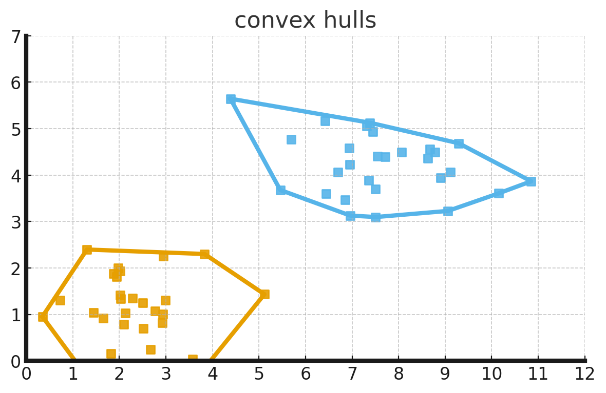
• the lines surrounding the outermost points of each class.
• since the classes are linearly separable, convex hulls do not intersect.

Margins

• the distance between data points of different classes seprarated by a hyperplane.
• multiple possible hyperplanes can separate the classes, but the optimal hyperplane maximizes the margin.
• Maximum Margin Hyperplane
  • a separation line/plane orthogonal to the shortest line connecting the convex hull.
  • the line that is farthest apart from each convex hull.
  • it separates the data points with the widest margin.

Kernels

• kernel is used to represent kernel functions
  • which are used to convert low-dimensional space to high-dimensional space
  • by applying a function on low-dimensional data points to come up with higher dimensions
    • which can be used to linearly separate the data points of classes using a hyperplane.
• the function of a kernel is to take data as input and transform it into the required form.
  • different algorithms use different types of kernel functions.
  • linear, non-linear, polynomial, radial basis function (RBF), and sigmoid.

Kernel trick

• Basic idea of SVM and Kernel trick is to find the plane which can separate, classify or split the data with maximum margin as possible.
• The distance from a point $(x_0, y_0)$ to a line $Ax + By + C = 0$ is given by the formula: $$\text{Distance} = \frac{|Ax_0 + By_0 + C|}{\sqrt{A^2 + B^2}}$$
• The distance between $H_0$, $H_1$ is then: $|w \cdot x + b| / ||w|| = 1/||w||$.
  • The total distance between $H_1$ and $H_2$ is $2/||w||$.
  • $H_1: w \cdot x + b = 1$
  • $H_2: w \cdot x + b = -1$.
  $$\text{Distance} = \frac{|(+1) - (-1)|}{||w||} = \frac{2}{||w||}$$
• to maximiza the margin, we need to minimize $||w||$
• this can be solved through Lagrangian formula or Lagrangian multipliers. $$L = \frac{1}{2} ||w||^2 - \sum_{i=1}^{n} \alpha_i [y_i (w \cdot x_i + b) - 1]$$
• Setting the gradient of $L$ $$\frac{\partial L}{\partial w} = 0 \Rightarrow w = \sum_{i=1}^{n} \alpha_i y_i x_i$$ $$\frac{\partial L}{\partial b} = 0 \Rightarrow \sum_{i=1}^{n} \alpha_i y_i = 0$$
• The dual form of the optimization problem is: $$\text{Maximize } W(\alpha) = \sum_{i=1}^{n} \alpha_i - \frac{1}{2} \sum_{i=1}^{n} \sum_{j=1}^{n} \alpha_i \alpha_j y_i y_j (x_i \cdot x_j)$$
• Capital letters such as A, X, Y denote matrices;
• Greek letters such as $\Phi$, $\kappa$ denote functions;
• lower-case bold letters such as $a$, $b$ denote vectors;
• script letters such as $\mathcal{A}$, $\mathcal{B}$, $\mathcal{V}$, $\mathcal{E}$ denote sets or spaces;
• $||a||$ denotes the $L^2$ norm of vector;
• $||x||_F$ denotes the Frobenius norm of matrix, and is given by $||x||_F = \big(\sum_{i,j} |x_{ij}|^2\big)^{1/2}$;

Linear Kernel

$K(x_i, x_j) = x_i \cdot x_j$

Gaussian Kernel / RBF Kernel

$K(x_i, x_j) = \exp\Big(-\frac{||x_i - x_j||^2}{2\sigma^2}\Big)$

Polynomial Kernel

$K(x_i, x_j) = (x_i \cdot x_j + 1)^h$

Sequential Minimal Optimization (SMO)

• an algorithm for solving the quadratic programming (QP) problem that arises during the training of support vector machines (SVMs).

Advantages

• Overfitting is unlikely
  • SVM uses the maximum margin hyperplane, which is relatively stable.
  • the maximum margin hyperplane is only sensitive to the changes in the support vectors.
  • the variance in the data may have a relatively low effect on the performance
• Computational complexity
  • since every time we need to classify a new sample we need to examine that sample with all the support vectors.
  • Using the kernel trick can help to alleviate this by calculating the dot product before doing the nonlinear mapping.

Disadvantages

• not perform very well when the data set has more noise
• where the number of features for each data point exceeds the number of training data samples, the SVM will underperform.

Applications

• Image classification
• Handwriting recognition
• Bioinformatics
• Text classification
• Top 10 SVM Applications