IAI +005
· 약 13분

Neural Network Development History
- 1950s-1960s: Early Foundations
- McCulloch & Pitts (1943): mathematical neuron model
- Rosenblatt's Perceptron (1958): first trainable network
- Minsky & Papert (1969): limitations (XOR problem) → AI Winter
- 1970s–1980s: First Revival
- Werbos (1974); Rumelhart, Hinton, Williams (1986): Backpropagation
- Hopfield Networks (1982): associative memory
- Renewed optimism but limited by hardware
- 1990s: Consolidation
- LeCun's CNN (LeNet, 1989): digit recognition
- Elman, Jordan: Recurrent Neural Networks
- Symbolic AI still dominated mainstream
- 2000s: Deep Learning Foundations
- Better hardware (GPUs) + large datasets
- Hinton (2006): Deep Belief Networks (unsupervised pretraining)
- Connectionism regains attention
- 2010s: Deep Learning Boom
- ImageNet (2012): AlexNet breakthrough
- RNNs, LSTMs, GRUs → speech & translation
- Transformers (2017): revolutionized NLP
- 2020s: Scaling & Foundation Models
- Large Language Models (GPT, BERT, etc.)
- Multimodal AI: vision, text, speech integration
- Connectionism dominates AI research & industry
Neural Network Models
- a collection of units (neurons) connected together
- The properties of the network are determined by its topology and the properties of the neurons.
- Roughly speaking, the neuron fires when a linear combination of its inputs exceeds some (hard or soft) threshold.
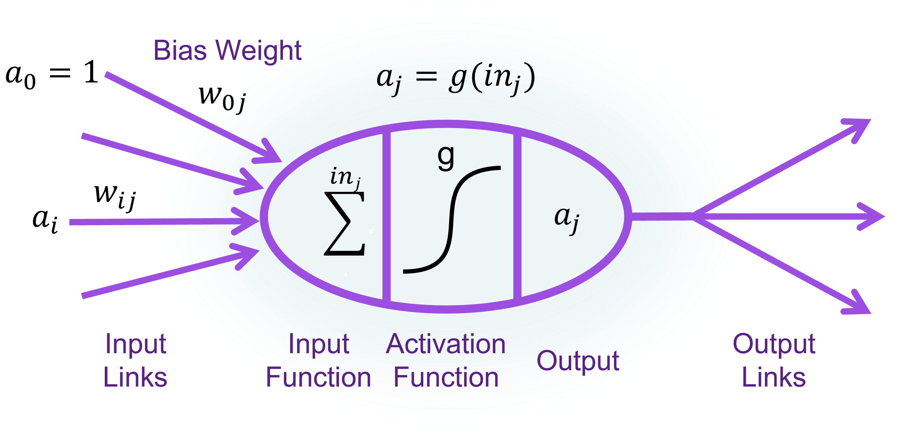
Activation function
ReLU function
- an abbreviation for rectified linear unit
- Commonly used
Softplus function
- A smooth version of the ReLU function
Logistic or Sigmoid function
- Non-linear, can represent a nonlinear function
Tanh function
Topology of a neural network
- Feed-forward network (FFN):
- Every node receives inputs from "upstream" nodes and delivers output to "downstream" nodes.
- There are no loops.
- FFN represents a function of its current inputs, thus it has no internal state other than the weights themselves.
- Recurrent Network (RNN):
- A recurrent network feeds its outputs back into its own inputs.
- In a recurrent network, the neuron values can eventually settle down, keep cycling, or behave unpredictably.
- can support short-term memory
| FFN | RNN |
|---|---|
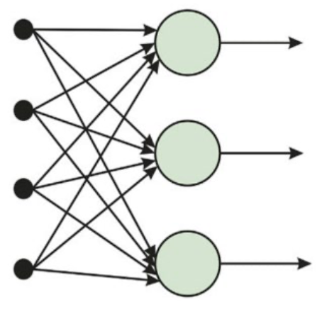 | 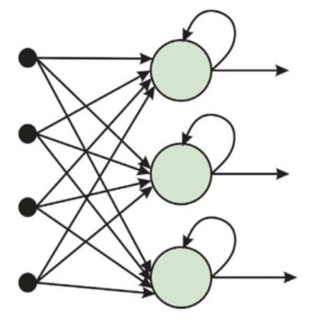 |
Training Process
- Go through each training sample.
- If correctly classified → do nothing.
- If misclassified → update the weights:
Perceptron for Binary Classification
- A perceptron separates data into two classes with a hyperplane.
- if
- if
Learning Rules
| Aspect | Perceptron Learning Rule | Gradient Descent (with Sigmoid) |
|---|---|---|
| Activation function | Hard threshold (계단 함수) | Sigmoid (연속 함수) |
| Output | 0 또는 1 | 0과 1 사이의 실수 값 |
| Loss function | 없음 (틀리면 조정, 맞으면 유지) 규칙 기반 학습 | (L2 loss) 또는 Cross-Entropy (실무에서 자주 사용) |
| Update rule | 틀렸을 때만: | 경사하강법: |
| Why derivative? | Hard threshold는 미분 불가능 → 단순 규칙 사용 | Sigmoid는 연속적이고 미분 가능 → Loss 함수의 기울기(gradient)를 따라 업데이트. 여기서 항은 sigmoid의 도함수에서 나온 것. |
| Interpretation | 틀리면 정답 방향으로 한 걸음 이동 | Loss가 줄어드는 방향으로 점진적으로 이동 |
Feadforward NN, FNN
- a multilayer perceptron network
- one input layer, N hidden layers,
N >= 1, and one output layer. - Except for the input layer, each layer has a same activation function
g. - The final output is represented by a vector function of inputs and weights.
- If it has three layers, Shallow Neural Network, otherwise Deep Neural Network.
Traning a FNN
- Forward
- Activation passing from the input layer to the output layer
- Calculate the output
- Backward
- Errors propagating backward from the output layer to the input layer
- Update weights
Forward phase
-
Activation of each node is computed in two steps:
- Weighted sum (in): sum of activations from the previous layer, multiplied by weights.
- Apply activation function g: pass the weighted sum through g to produce the node's activation.
-
Process: propagate activations layer by layer towards the output layer.
-
Output value (example with 2 layers):
Backward phase
- Loss function: choose squared error loss (L2)
- Prediction:
- Gradient descent: compute gradient of the loss with respect to weights, then update weights along the negative gradient direction.
- Example: sigmoid activation:
- Gradient of the loss:
- Chain rule applied:
- Example: Gradient derivation for sigmoid
- Weighted input
- (where for the bias)
- Gradient of the loss
- Derivative of sigmoid output
-
- Derivative of weighted input
- Weight update rule
- General form:
- Weighted input
Backward phase Steps
- Select a loss function
- For example, squared error loss:
- Choose an activation function
- Suppose we use a sigmoid:
- Calculate the error at the output node
- The delta (error term) at the output is
- Calculate the error at hidden nodes
- A hidden unit may connect to multiple nodes in the next layer.
- Therefore, its error is the weighted sum of all deltas it feeds into, scaled by its own derivative:
- The summation appears because the hidden node's output influences several downstream nodes, and all those error signals must be aggregated.
- Update the weights with gradient descent
- The gradient with respect to weight is simply the input times the delta:
- Update rule:
Vanishing gradient
- The error signal are extinguished altogher as they are propagated back through the network
- In deep feedforward networks with
sigmoid/tanh, repeated multiplication of small derivatives () during backpropagation causes the gradient to vanish.
Optimizer
- Training a neural network consists of modifying the network's parameters, minimizing the loss function on the training set.
- any kind of optimization algorithm could be used.
- modern neural networks are almost always trained with some variant of stochastic gradient descent (SGD). Adam Optimizer
- The optimiser is specified in the compilation step with tensorflow.
Recurrent NN, RNN
- units may take as input a value computed from their own output at an earlier step in the computation.
- have internal state, or memory: inputs received at earlier time steps affect the RNN's response to the current input.
- be used to perform more general computations.
- to analyze sequential data in which a new input vector arrives at each time step
- Markov assumption: the hidden state of the network suffices to capture the information from all previous inputs.
- Once trained, this function represents a time-homogeneous process
- The same update rule applies at every time step, regardless of whether it’s the first input or the hundredth.
- RNNs are designed for sequential data.
- a hidden state that captures information from previous steps.
- suffer from vanishing/exploding gradients.
- Good for short-term dependencies.
Backpropagtion Through Time, BPTT
- gradient expression is recursive.
-
- includes
- the gradient with run time being linear in the size of the network
- handled automatically by deep learning software systems.
- Iterating the recursion shows that the gradient at time includes a term proportional to:
- Since for sigmoid, tanh, and ReLU we have , if the RNN will suffer from the vanishing gradient problem.
- If , we may encounter the exploding gradient problem.
Long Short-Term Memory, LSTM
- memory cell is essentially copied from time step to time step.
- New information enters the memory by adding updates.
- the gradient expressions do not accumulate multiplicatively over time.
- include gating units: vectors control the flow of information in the LSTM, elementwise multiplication of the corresponding information vector.
- a type of RNN designed to overcome vanishing gradient.
- use gates (input, forget, output) to control information flow.
- Capable of learning long-term dependencies.
- Widely used in NLP, speech recognition, and time series forecasting.
Gates in LSTM
- Forget gate: decides what information to discard from the cell state.
- Input gate: decides what new information to store in the cell state.
- Output gate: decides what information to output from the cell state.
- similar role to the hidden state in basic RNNs.
- Update equations:
-
- Decides which parts of the previous cell state should be kept or discarded.
-
- Determines how much of the new information from the current input and the previous hidden state should be added.
-
- Controls which parts of the current cell state are exposed as the hidden state .
-
- Cell state update
- Past information () is partially retained through the forget gate.
- New information is added through the input gate and .
- Thus, serves as the long-term memory of the LSTM.
-
- Hidden state update
- The cell state is normalized with and filtered by the output gate.
- is the hidden state passed forward to the next time step.
-
Gated Recurrent Unit, GRU
- Variant of RNN with gating mechanisms.
- Designed to capture long-term dependencies without complex architecture.
- a simpler alternative to LSTMs. (lightweight, effective RNN variant)
- Captures temporal dependencies (short & long).
- Combine input and forget gates into a single update gate.
- Require fewer parameters than LSTM, making them faster to train.
- Perform comparably to LSTMs in many tasks.
- Prevents vanishing gradient.
- Good balance between complexity & performance.
- Excels in time series forecasting tasks.
- Widely used in finance, energy and IoT.
Gates in GRU
- Update gate (z): decides how much past information to keep
- Reset Gate (r): decides how much past information to forget
- Candidate hidden state (): potential new memory
- Final hidden state (): weighted combination of old and new information.
GRU Workflow
- Reset gate ()
- Controls how much of the previous hidden state should be "forgotten."
- A small value means most of the past memory is erased, while a large value means much of it is retained.
- Update gate ()
- Acts as a switch to decide whether to keep the previous state or replace it with the new candidate .
- If , the past is fully kept; if , it is completely replaced by the new candidate.
- Candidate state ()
- Combines the current input with the reset-gated previous hidden state to generate the "candidate" new information.
- Final hidden state ()
- Blends the past and the candidate using the update gate .
- If is large → the past memory dominates.
- If is small → the new candidate dominates.
Comparison: RNN vs LSTM vs GRU
| Attribute | RNN | LSTM | GRU |
|---|---|---|---|
| Architecture | Simple, hidden state | Complex, memory cell + 3 gates | Simplified, 2 gates (update/reset) |
| Information Flow | Stored in hidden state | Controlled by gates | Controlled by merged gates |
| Long-term Dependency | Weak (vanishing gradient) | Strong (gates solve vanishing gradient) | Strong (gates solve vanishing gradient) |
| Short-term Dependency | Strong | Strong | Strong |
| Number of Parameters | Few | Many | Fewer than LSTM |
| Training Speed | Fast | Slow | Fast |
| Performance | Good for short-term | Good for long-term | Efficient, similar to LSTM |
| Application Areas | Simple time series, basic NLP | NLP, speech, time series forecasting | Finance, IoT, energy, time series |
| Vanishing Gradient | Yes | No | No |
| Typical Use Cases | Text generation, simple prediction | Translation, speech recognition | Time series prediction, sensor data |
| Simplicity | Very simple, rarely used | More complex, expressive (3 gates) | Simpler than LSTM, fewer parameters |
| Expressiveness | Limited, struggles with long-term | High, handles very complex sequences | Moderate, good for moderate data size |
| Training Efficiency | Fast, but limited | Slower, better for complex data | Fast, efficient, similar performance |
| Trade-off | Simple but weak for long-term | Capacity for complex, long sequences | Simplicity vs. capacity |