IAI +003
· 약 5분

Local Search Problem
To find the state that gives the optimal/best value of the evaluation function
- It can be seen as an optimization problem.
- a computational problem that finds the best solution (a state) that satisfies the given constraints
evaluation function === objective function- Only cares about the optimal solution/best state without considering the paths to reach the best state (the optimal solution)
- Not systematic
Feasible region & solution
- Feasible region: the set of all possible or candidate solutions which are the solutions that satisfies the problem's constraints
- Feasible solution: a solution in the feasible region
Search Problem vs Local Search Problem
Path-based vs State-based
| Aspects | Search Problem | Local Search Problem |
|---|---|---|
| State | All possible states - state-space landscape | Range of decision variables and constraints |
| Goal | Goal state & goal test | Evaluation function & objective function |
| Evaluation | Measure closeness to goal - distance/fitness | Minimize cost or maximize fitness |
| Transition/Successor | Transition function | Successor function |
Discrete & Continuous Optimization
- Discrete optimization: optimization problems where the solution space is discrete (e.g., 8 queens problem)
- Continuous optimization: optimization problems where the solution space is continuous (e.g., real numbers, any value within a range)
Information needed for Local Search
- All possible states: state-space landscape
- Transition function: To find neighbor or successor state
- Goal state
- Objective function: A way to measure how close to the goal state
- Start state
Search state-space
- Global Maximum: A state that maximizes the objective function over the entire state space
- Local Maximum: A state that maximizes the objective function within a small area around it.
- Plateau: A state such that the objective function is constant in an area around it.
- Shoulder: A plateau that has uphill edge.
- Flat: A plateau whose edges go downhill.
Advantages
- use little memory
- can often find reasonably good solution in large or infinite search spaces
- useful for solving pure optimization problems
- don't need to know the path to the solution.
Hill climbing
keeps track of one current state and on each iteration moves to the neighboring state with highest value.
- Steps
- Evaluate the initial stat
- If it is equal to the goal state, return. Otherwise, continue.
- Find a neighboring state
- Evaluate this state. If it is closer to the goal state than before, replace the initial state with this state.
- Repeat steps 2-4 until it reaches a goal state (local or global maximum) or runs out of time.
- No search tree, No backtracking, Don't look ahead beyond the current state.
- get stuck due to local maxima, plateaus, or ridges.
Variations of HC
- Simple HC: greedy local search which expands the current state and moves on to the best neighbor.
- Stochastic HC: choose randomly among the neighbors going uphill.
- First-choice HC: generate random successor until one is better. Good for states with high numbers of successors.
- Random restart: conducts a series of hill climbing searches from random initial states until a goal state is found.
Simulated Annealing
based upon the annealing process to model the search process for finding an optimal solution to an optimisation problem
- annealing schedule, temperature, energy
- finds the minimal value of the objective function (energy function)
- starts with a high temperature and then gradually reduces the temperature
-
- : how bad the new state is compared to the old state
- : temperature is getting lower over time
- : a scaling factor
- Swap condition: or
Evolutionary algorithms
- Local beam search
- Stochastic beam search
- Genetic algorithms
Characteristics
- size of the population
- representation of each individual
- mixing number
- selection process for selecting the individuals who will become the parents of the next generation
- recombination procedure
- mutation rate
- makeup of the next generation
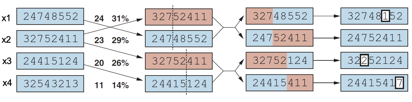
Genetic algorithm
It uses operators, such reproduction, crossover and mutation, inspired by the natural evolutionary principles.
- State: is represented by an individual in a population. Traditional representation is a chromosome
- Objective function: is used to evaluate the fitness of an individual (= fitness function, 적합도 함수)
- Successor function: consists of three operators: reproduction, crossover, and mutation
- Solution: is found through evolution from one generation to another generation
Roulette Wheel Selection
- Compute total fitness of all individuals.
- Example: A=30, B=20, C=40, D=10 → Total = 100.
- Calculate probability of each individual being selected
- Formula:
- A = 30/100 = 0.30
- B = 20/100 = 0.20
- C = 40/100 = 0.40
- D = 10/100 = 0.10
- Formula:
- Convert to cumulative probabilities
- P4 = 0.10
- P4 + P3 = 0.50
- P4 + P3 + P2 = 0.90
- P4 + P3 + P2 + P1 = 1.00
- Generate a random number between 0 and 1.
- Select an individual based on the random number and cumulative probabilities.
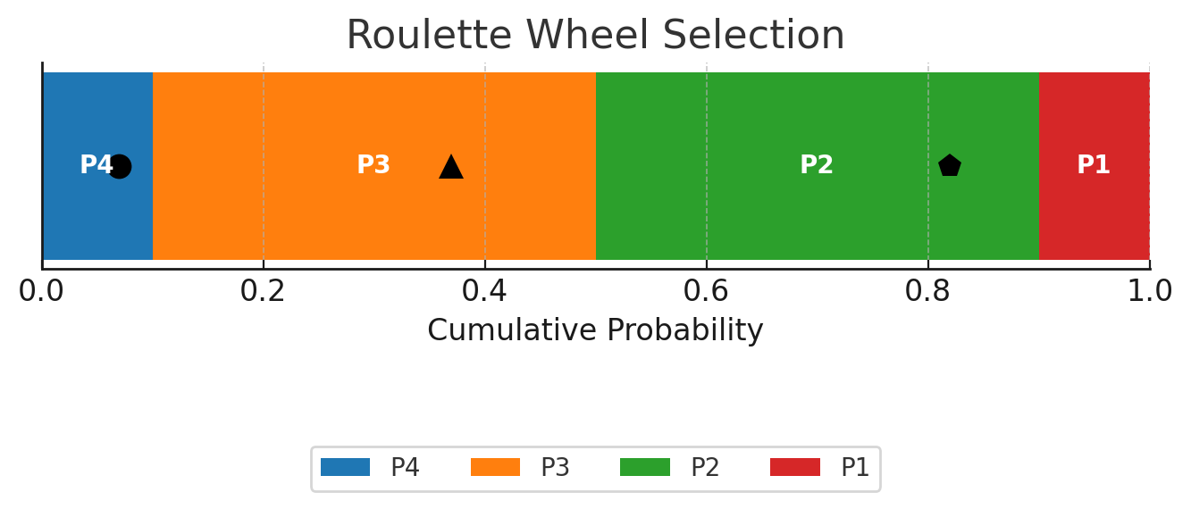
- ⚫ random = 0.07 → falls in P4
[0, 0.10) - 🔺 random = 0.37 → falls in P3
[0.10, 0.50) - ⬟ random = 0.82 → falls in P2
[0.50, 0.90)
Applications of GA
- Parameter tuning: optimize the parameters in NN
- Planning: economic dispatch, train timetabling
- Design & Control problems: robotic control, adaptive control systems
- Successful use of GA requires careful engineering of the representation